MacroPlacement
Our Progress: A Chronology
Table of Contents
- Introduction
- Our progress and major milestones
- Publicly available commercial SP&R flow
- Ariane133 macro placement using Circuit Training
- Replication of proxy cost
- NVDLA macro placement using Circuit Training
- BlackParrot (Quad Core) macro placement using Circuit Training
- Circuit Training stability study
- Proxy cost correlation study
- MemPool Group macro placement using Circuit Training
- Macro placement on GLOBALFOUNDRIES 12 nm enablement
- Macro placement using AutoDMP
- Macro placement generated using Simulated Annealing
- Macro placement by Human expert
- Macro placement using Hier-RTLMP
- Protobuf to LEF/DEF and macro placement of CT-Ariane
- Pinned questions
Introduction
MacroPlacement is an open, transparent effort to provide a public, baseline implementation of Google Brain’s Circuit Training (Morpheus) deep RL-based placement method. In this repo, we aim to achieve the following.
- We want to enable anyone to perform RL-based macro placement on their own design, starting from design RTL files.
- We want to enable anyone to train their own RL models based on their own designs in any design enablements, starting from design RTL files.
- We want to demystify important aspects of the Google Nature paper, including aspects unavailable in Circuit Training and aspects where the Nature paper and Circuit Training clearly diverge, in order to help researchers and users better understand the methodology.
- We want to apply learnings from the community’s collective experiences with the Google Brain team’s arXiv result, Nature paper and Circuit Training repo – and demonstrate how communication of research results might be improved in our community going forward. A clear theme from the past months’ experience: “There is no substitute for source code.”
In order to achieve the above goals, our initial focus has been on the following efforts.
- Generating correct inputs and setup for Circuit Training. Since Circuit Training uses protocol buffer format to represent designs, we must translate standard LEF/DEF representation to the protocol buffer format. We must also determine how to correctly feed all necessary design information into the Google Brain’s Circuit Training flow, e.g., halo width, canvas size, and constraints. If we accomplish this, then we can run Google Brain’s Circuit Training to train our own RL models or perform RL-based macro placement for our own designs.
- Replicating important but missing parts of the Google Nature paper. Several aspects of Circuit Training are not clearly documented in the Nature paper, nor in the code and scripts that are visible in Circuit Training. Over time, these have included hypergraph-to-graph conversion; gridding, grouping and clustering; force-directed placement; various hyperparameter settings; and more. As we keep moving forward, based on our experiments and continued Q&A and feedback from Google, we will summarize the miscorrelations between the Google Nature paper and Google Brain’s Circuit Training, as well as corrective steps. In this way, the Circuit Training methodology and the results published in the Nature paper can be better understood by all.
Our Progress
June 6 - Aug 5: We have developed and made publicly available the SP&R flow using commercial tools Cadence Genus and Innovus, and open-source tools Yosys and OpenROAD, for Ariane (two variants – one with 136 SRAMs and another with 133 SRAMs), MemPool tile and NVDLA designs on NanGate45, ASAP7 and SKY130HD open enablement. We applaud and thank Cadence Design Systems for allowing their tool runscripts to be shared openly by researchers, enabling reproducibility of results obtained via use of Cadence tools. This was an important milestone for the EDA research community. Please see Dr. David Junkin’s presentation at the recent DAC-2022 “Open-Source EDA and Benchmarking Summit” birds-of-a-feather meeting.
The following describes our learning related to testcase generation and its implementation using different tools on different platforms.
- The Google Nature paper uses the Ariane testcase (contains 133 256x16-bit SRAMs) for their experiment. Here we show that just instantiating 256x16 bit SRAMs results in 136 SRAMs in the synthesized netlist. Based on our investigations, we have provided the detailed steps to convert the Ariane design with 136 SRAMs to a Ariane design with 133 SRAMs.
- We provide the required SRAM lef, lib along with the description to reproduce the provided SRAMs or generate a new SRAM for each enablement.
- The SKY130HD enablement has only five metal layers, while SRAMs have routing up through the M4 layer. This causes P&R failure due to very high routing congestion. We therefore developed FakeStack-extended P&R enablement, where we replicate the first four metal layers to generate a nine metal layer enablement. We call this SKY130HD-FakeStack and have used it to implement our testcases. We also provide a script for researchers to generate FakeStack enablements with different configurations.
- We provide power grid generation scripts for Cadence Innovus. During the power grid (PG) generation process we made sure the routing resource used by the PG is in the range of ~20%, matching the guidance given in Circuit Training.
- Also we provide an Innovus Tcl script to extract the metrics reported in Table 1 of “A graph placement methodology for fast chip design”, at three stages of the post-floorplanning P&R flow, i.e., pre-CTS, post-CTSOpt, and post-RouteOpt (final). This script is included in the P&R flow. The extracted metrics for all of our designs, on different enablements, are available here.
June 10: grouper.py was released in CircuitTraining. This revealed that protobuf input to the hypergraph clustering into soft macros included the (x,y) locations of the nodes. (A grouper.py script had been shown to Prof. Kahng during a meeting at Google on May 19.) The use of (x,y) locations from a physical synthesis tool was very unexpected, since it is not mentioned in “Methods” or other descriptions given in the Nature paper. We raised issue #25 to get clarification about this. [July 10: The README added to the grouping area of CircuitTraining confirmed that the input netlist has all of its nodes already placed.]
We currently use the physical synthesis tool Cadence Genus iSpatial to obtain (x,y) placed locations per instance as part of the input to Grouping. The Genus iSpatial post-physical-synthesis netlist is the starting point for how we produce the clustered netlist and the *.plc file which we provide as open inputs to CircuitTraining. From post-physical-synthesis netlist to clustered netlist generation can be divided into the following steps, which we have implemented as open-source in our CodeElements area:
- June 6: Gridding determines a dissection of the layout canvas into some number of rows and some number of columns of gridcells.
- June 10: Grouping groups closely-related logic with the corresponding hard macros and clumps of IOs.
- June 12: Clustering clusters of millions of standard cells into a few thousand clusters (soft macros).
June 22: We added our flow-scripts that run our gridding, grouping and clustering implementations to generate a final clustered netlist in protocol buffer format. Google’s netlist protocol buffer format documentation available in the CircuitTraining repo was very helpful to our understanding of how to convert a placed netlist to protobuf format. Our scripts enable clustered netlists in protobuf format to be produced from placed netlists in either LEF/DEF or Bookshelf format.
July 12: As stated in the “What is your timeline?” FAQ response [see also note [5] here], we presented progress to date in this MacroPlacement talk at the DAC-2022 “Open-Source EDA and Benchmarking Summit” birds-of-a-feather meeting.
July 26: Replication of the wirelength component of proxy cost. The wirelength is similar to HPWL where given a netlist, we take the width and height and sum them up for each net. One caveat is that for soft macro pins, there could be a weight factor which implies the total connections between the source and sink pins. If not defined, the default value is 1. This weight factor needs to be multiplied with the sum of width and height to replicate Google’s API. We provide the following table as a comparison between our implementations and Google’s API.
| Testcase | Notes | Canvas width/height | Grid col/row | Our | |
|---|---|---|---|---|---|
| Ariane | Google’s Ariane | 356.592 / 356.640 | 35 / 33 | 0.7500626080261634 | 0.7500626224300161 |
| Ariane133 | From MacroPlacement | 1599.99 / 1598.8 | 50 / 50 | 0.6522555375409593 | 0.6522555172428797 |
July 31: The netlist protocol buffer format documentation also helped us to write this Innovus-based tcl script which converts physical synthesized netlist to protobuf format in Innovus. [This script was written and developed by ABKGroup students at UCSD. However, the underlying commands and reports are copyrighted by Cadence. We thank Cadence for granting permission to share our research to help promote and foster the next generation of innovators.] We use this post-physical-synthesis protobuf netlist as input to the grouping code to generate the clustered netlist. Fixes that we made while running Google’s grouping code resulted in this [08/01/2022] pull request. [08/05/2022: Google’s grouping code has been updated based on this PR.]
July 22-August 4: We shared with Google engineers our (flat) post-physical-synthesis-protobuf netlist (ariane.pb.txt) of our Ariane design with 133 SRAMs on the NanGate45 platform, along with the corresponding clustered netlist and the legalized.plc file (clustered netlist: netlist.pb.txt) generated using the CircuitTraining grouping code. The goal here was to verify our steps and setup up to this point. Also, we provide scripts (using both our CodeElements and CT-grouping) to integrate the clustered netlist generation with the SP&R flow.
August 5: The following table compares the clustering results for Ariane133-NG45 design generated by the Google engineer (internally to Google) and the clustering results generated by us using CT grouping code.
| Google Internal flow (from Google) | Our use of CT Grouping code | |
|---|---|---|
| Number of grid rows x columns | 21 x 24 | 21 x 24 |
| Number of soft macros | 736 | 738 |
| HPWL | 4171594.811 | 4179069.884 |
| Wirelength cost | 0.072595 | 0.072197 |
| Congestion cost | 0.727798 | 0.72853 |
August 11: We received information from Google that when a standard cell has multiple outputs, it merges all of them in the protobuf netlist (example: a full adder cell would have its outputs merged). The possible vertices of a hyperedge are macro pins, ports, and standard cells. Our Innovus-based protobuf netlist generation tcl script takes care of this.
August 15: We received information from Google engineers that in the proxy cost function, the density weight is set to 0.5 for their internal runs.
August 17: The proxy wirelength cost which is usually a value between 0 and 1, is related to the HPWL we computed earlier. We deduce the formulation as the following:

|netlist| is the total number of nets and it takes into account the weight factor defined on soft macro pins. Here is our proxy wirelength compared with Google’s API:
| Testcase | Notes | Canvas width/height | Our | |
|---|---|---|---|---|
| Ariane | Google’s Ariane | 356.592 / 356.640 | 0.05018661999974192 | 0.05018662006439473 |
| Ariane133 | From MacroPlacement | 1599.99 / 1598.8 | 0.04456188308735019 | 0.04456188299072617 |
Replication of the density component of proxy cost. We now have a verified density cost computation. Density cost computation depends on gridcell density. Gridcell density is the ratio of the total area occupied by standard cells, soft macros and hard macros to the total area of the grid. If there are cell overlaps then it may result in grid density greater than one. To get the density cost, we take the average of the top 10% of the densest gridcells. Before outputting it, we multiply it by 0.5. Notice that this 0.5 is not the “weight” of this cost function, but simply another factor applied besides the weight factor from the cost function.

| Testcase | Notes | Canvas width/height | Grid col/row | Our | |
|---|---|---|---|---|---|
| Ariane | Google’s Ariane | 356.592 / 356.640 | 35 / 33 | 0.7500626080261634 | 0.7500626224300161 |
| Ariane133 | From MacroPlacement | 1599.99 / 1598.8 | 50 / 50 | 0.6522555375409593 | 0.6522555172428797 |
August 18: The flat post-physical-synthesis protobuf netlist of Ariane133-NanGate45 design is used as input to CT grouping code to generate the clustered netlist. We then use this clustered netlist in Circuit Training. Coordinate Descent is (by default) not applied to any macro placement solution. Here is the link to our tensorboard. We ran Innovus P&R starting from the macro placement generated using CT, through the end of detailed routing (RouteOpt) and collection of final PPA / “Table 1” metrics. Following are the metrics and screen shots of the P&R database. Throughout the SP&R flow, the target clock period is 4ns. The power grid overhead is 18.46% in the actual P&R setup, matching the 18% mentioned in the Circuit Training repo. All results are for DRC-clean final routing produced by the Innovus tool.
[In the immediately-following content, we also show comparison results using other macro placement methods, collected since August 18.]
[As of August 24 onward, we refer to this testcase as “Our Ariane133-NanGate45_51” since it has 51% area utilization. A second testcase, “Our Ariane133-NanGate45_68”, has 68% area utilization which exactly matches that of the Ariane in Circuit Training.]
Circuit Training Baseline Result on “Our Ariane133-NanGate45_51”.
Macro placement generated by Circuit Training on Our Ariane-133 (NG45), with post-macro placement flow using Innovus21.1 |
|||||||||
|---|---|---|---|---|---|---|---|---|---|
| Physical Design Stage | Core Area (um^2) | Standard Cell Area (um^2) | Macro Area (um^2) | Total Power (mW) | Wirelength (um) | WS (ns) |
TNS (ns) |
Congestion (H) | Congestion (V) |
| preCTS | 2560080 | 214555 | 1018356 | 287.79 | 4343214 | 0.005 | 0 | 0.01% | 0.02% |
| postCTS | 2560080 | 216061 | 1018356 | 301.31 | 4345969 | 0.010 | 0 | 0.01% | 0.02% |
| postRoute | 2560080 | 216061 | 1018356 | 300.38 | 4463660 | 0.359 | 0 | ||


Comparison 1: “Human Gridded”. For comparison, a baseline “human, gridded” macro placement was generated by a human for the same canvas size, I/O placement and gridding, with results as follows.
Macro placement generated by a human on Our Ariane-133 (NG45), with post-macro placement flow using Innovus21.1 |
|||||||||
|---|---|---|---|---|---|---|---|---|---|
| Physical Design Stage | Core Area (um^2) | Standard Cell Area (um^2) | Macro Area (um^2) | Total Power (mW) | Wirelength (um) | WS (ns) |
TNS (ns) |
Congestion (H) | Congestion (V) |
| preCTS | 2560080 | 215188.9 | 1018356 | 285.96 | 4470832 | -0.002 | -0.005 | 0.00% | 0.00% |
| postCTS | 2560080 | 216322.9 | 1018356 | 299.62 | 4472866 | 0.001 | 0 | 0.00% | 0.00% |
| postRoute | 2560080 | 216322.9 | 1018356 | 298.60 | 4587141 | 0.284 | 0 | ||

Comparison 2: RePlAce. The standalone RePlAce placer was run on the same (flat) netlist with the same canvas size and I/O placement, with results as follows.
Macro placement generated by RePlAce (standalone, from HERE) on Our Ariane-133 (NG45), with post-macro placement flow using Innovus21.1 |
|||||||||
|---|---|---|---|---|---|---|---|---|---|
| Physical Design Stage | Core Area (um^2) | Standard Cell Area (um^2) | Macro Area (um^2) | Total Power (mW) | Wirelength (um) | WS (ns) |
TNS (ns) |
Congestion (H) | Congestion (V) |
| preCTS | 2560080 | 214910.71 | 1018356 | 288.654 | 4178509 | 0.003 | 0 | 0.03% | 0.07% |
| postCTS | 2560080 | 216006.63 | 1018356 | 302.013 | 4184690 | 0.007 | 0 | 0.05% | 0.08% |
| postRoute | 2560080 | 216006.63 | 1018356 | 301.260 | 4315157 | -0.207 | -0.41 | ||


Comparison 3: RTL-MP. The RTL-MP macro placer described in this ISPD-2022 paper and used as the default macro placer in OpenROAD was run on the same (flat) netlist with the same canvas size and I/O placement, with results as follows.
Macro placement generated using RTL-MP on Our Ariane-133 (NG45), with post-macro placement flow using Innovus21.1 |
|||||||||
|---|---|---|---|---|---|---|---|---|---|
| Physical Design Stage | Core Area (um^2) | Standard Cell Area (um^2) | Macro Area (um^2) | Total Power (mW) | Wirelength (um) | WS (ns) |
TNS (ns) |
Congestion (H) | Congestion (V) |
| preCTS | 2560080 | 216420.26 | 1018356 | 289.435 | 5164199 | 0.020 | 0 | 0.04% | 0.05% |
| postCTS | 2560080 | 217938.32 | 1018356 | 303.757 | 5185004 | 0.001 | 0 | 0.05% | 0.07% |
| postRoute | 2560080 | 217938.32 | 1018356 | 302.844 | 5306735 | 0.104 | 0 | ||


Comparison 4: The Hier-RTLMP macro placer was run on the same (flat) netlist with the same canvas size and I/O placement, with results as follows. [The Hier-RTLMP paper is in submission as of August 2022; availability in OpenROAD and OpenROAD-flow-scripts is planned by end of September 2022. Please email abk@eng.ucsd.edu if you would like a preprint, not for further redistribution.]
Macro placement generated using Hier-RTLMP on Our Ariane-133 (NG45), with post-macro placement flow using Innovus21.1 |
|||||||||
|---|---|---|---|---|---|---|---|---|---|
| Physical Design Stage | Core Area (um^2) | Standard Cell Area (um^2) | Macro Area (um^2) | Total Power (mW) | Wirelength (um) | WS (ns) |
TNS (ns) |
Congestion (H) | Congestion (V) |
| preCTS | 2560080 | 214783.83 | 1018356 | 288.356 | 4397005 | 0.005 | 0 | 0.02% | 0.05% |
| postCTS | 2560080 | 215911.67 | 1018356 | 302.176 | 4419305 | 0.009 | 0 | 0.04% | 0.06% |
| postRoute | 2560080 | 215911.67 | 1018356 | 301.468 | 4537458 | 0.311 | 0 | ||


August 20: Matching the area utilization. We revisited the area utilization of Our Ariane133 and realized that it (51%) is lower than that of Google’s Ariane (68%). So that this would not devalue our study, we created a second variant, “Our Ariane133-NanGate45_68”, which matches the area utilization of Google’s Ariane. Results are as given below.
Circuit Training Baseline Result on “Our Ariane133-NanGate45_68”.
| Physical Design Stage | Core Area (um^2) | Standard Cell Area (um^2) | Macro Area (um^2) | Total Power (mW) | Wirelength (um) | WS (ns) |
TNS (ns) |
Congestion (H) | Congestion (V) |
| preCTS | 1814274 | 215575.444 | 1018355.73 | 288.762 | 4170253 | 0.002 | 0 | 0.01% | 0.01% |
| postCTS | 1814274 | 217114.520 | 1018355.73 | 302.607 | 4186888 | 0.001 | 0 | 0.00% | 0.01% |
| postRoute | 1814274 | 217114.520 | 1018355.73 | 301.722 | 4295572 | 0.336 | 0 | ||


Comparison 1: “Human Gridded”. For comparison, a baseline “human, gridded” macro placement was generated by a human for the same canvas size, I/O placement and gridding.
Macro Placement generated by human (Util: 68%) |
|||||||||
|---|---|---|---|---|---|---|---|---|---|
| Physical Design Stage | Core Area (um^2) | Standard Cell Area (um^2) | Macro Area (um^2) | Total Power (mW) | Wirelength (um) | WS (ns) |
TNS (ns) |
Congestion (H) | Congestion (V) |
| preCTS | 1814274 | 215779 | 1018355.73 | 289.999 | 4545632 | -0.003 | -0.004 | 0.09% | 0.15% |
| postCTS | 1814274 | 217192 | 1018355.73 | 303.786 | 4571293 | 0.001 | 0 | 0.13% | 0.16% |
| postRoute | 1814274 | 217192 | 1018355.73 | 302.725 | 4720776 | 0.206 | 0 | ||


Comparison 2: RePlAce. The standalone RePlAce placer was run on the same (flat) netlist with the same canvas size and I/O placement, with results as follows.
Macro Placement generated Using RePlAce (Util: 68%) |
|||||||||
|---|---|---|---|---|---|---|---|---|---|
| Physical Design Stage | Core Area (um^2) | Standard Cell Area (um^2) | Macro Area (um^2) | Total Power (mW) | Wirelength (um) | WS (ns) |
TNS (ns) |
Congestion (H) | Congestion (V) |
| preCTS | 1814274 | 217246 | 1018355.73 | 292.803 | 4646408 | -0.007 | -0.011 | 0.07% | 0.13% |
| postCTS | 1814274 | 218359 | 1018355.73 | 306.145 | 4657174 | 0.001 | 0 | 0.07% | 0.17% |
| postRoute | 1814274 | 218359 | 1018355.73 | 305.032 | 4809950 | 0.082 | 0 | ||


Comparison 3: RTL-MP. The RTL-MP macro placer was run on the same (flat) netlist with the same canvas size and I/O placement, with results as follows.
Macro Placement generated Using RTL-MP (Util: 68%) |
|||||||||
|---|---|---|---|---|---|---|---|---|---|
| Physical Design Stage | Core Area (um^2) | Standard Cell Area (um^2) | Macro Area (um^2) | Total Power (mW) | Wirelength (um) | WS (ns) |
TNS (ns) |
Congestion (H) | Congestion (V) |
| preCTS | 1814274 | 217057 | 1018355.73 | 292.800 | 4598656 | -0.001 | -0.001 | 0.00% | 0.01% |
| postCTS | 1814274 | 218045 | 1018355.73 | 306.475 | 4614827 | 0.007 | 0 | 0.00% | 0.01% |
| postRoute | 1814274 | 218045 | 1018355.73 | 303.380 | 4745004 | 0.294 | 0 | ||


Comparison 4: The Hier-RTLMP macro placer was run on the same (flat) netlist with the same canvas size and I/O placement, using two setups, with results as follows.
Macro Placement generated Using Hier-RTLMP (Util: 68%) [Setup 1] |
|||||||||
|---|---|---|---|---|---|---|---|---|---|
| Physical Design Stage | Core Area (um^2) | Standard Cell Area (um^2) | Macro Area (um^2) | Total Power (mW) | Wirelength (um) | WS (ns) |
TNS (ns) |
Congestion (H) | Congestion (V) |
| preCTS | 1814274 | 218096 | 1018355.73 | 294.035 | 4967286 | 0.003 | 0 | 0.10% | 0.12% |
| postCTS | 1814274 | 219150 | 1018355.73 | 308.130 | 4984385 | 0.001 | 0 | 0.13% | 0.13% |
| postRoute | 1814274 | 219150 | 1018355.73 | 307.103 | 5137430 | 0.387 | 0 | ||


Macro Placement generated Using Hier-RTLMP (Util: 68%) [Setup 2] |
|||||||||
|---|---|---|---|---|---|---|---|---|---|
| Physical Design Stage | Core Area (um^2) | Standard Cell Area (um^2) | Macro Area (um^2) | Total Power (mW) | Wirelength (um) | WS (ns) |
TNS (ns) |
Congestion (H) | Congestion (V) |
| preCTS | 1814274 | 216665 | 1018355.73 | 291.332 | 4917102 | 0.001 | 0 | 0.02% | 0.06% |
| postCTS | 1814274 | 217995 | 1018355.73 | 305.089 | 4931432 | 0.001 | 0 | 0.03% | 0.05% |
| postRoute | 1814274 | 217995 | 1018355.73 | 303.905 | 5048575 | 0.230 | 0 | ||


August 25: Replication of the congestion component of proxy cost. Reverse-engineering from the plc client API is finally completed, as described here. A review with Dr. Mustafa Yazgan was very helpful in confirming the case analysis and conventions identified during reverse-engineering. Replication results are shown below. With this, reproduction in open source code of the Circuit Training proxy cost has been completed. Note that the description here illustrates how the Nature paper, Circuit Training, and Google engineers’ versions can have minor discrepancies. (These minor discrepancies are not currently viewed as substantive, i.e., meaningfully affecting our ongoing assessment.) For example, to calculate the congestion component, the H- and V-routing congestion cost lists are concatenated, and the ABU5 (average of top 5% of the concatenated list) metric of this list is the congestion cost. By contrast, the Nature paper indicates use of an ABU10 metric. Recall: “There is no substitute for source code.”
| Name | Description | Canvas Size | Col/Row | Congestion Smoothing | Google’s Congestion | Our Congestion |
|---|---|---|---|---|---|---|
| Ariane | Google’s Ariane | 356.592 / 356.640 | 35 / 33 | 0 | 3.385729893179586 | 3.3857299314069733 |
| Ariane133 | Our Ariane | 1599.99 / 1600.06 | 24 / 21 | 0 | 1.132108622298701 | 1.1321086382282062 |
| Ariane | Google’s Ariane | 356.592 / 356.640 | 35 / 33 | 1 | 2.812822828059799 | 2.81282287498789 |
| Ariane133 | Our Ariane | 1599.99 / 1600.06 | 24 / 21 | 1 | 1.116203573147857 | 1.1162035989647672 |
| Ariane | Google’s Ariane | 356.592 / 356.640 | 35 / 33 | 2 | 2.656602005772668 | 2.6566020148393146 |
| Ariane133 | Our Ariane | 1599.99 / 1600.06 | 24 / 21 | 2 | 1.109241385529823 | 1.1092414113467333 |
August 26: Moving on to understand benefits and limitations of the Circuit Training methodology itself. This next stage of study is enabled by confidence in the technical solidity of what has been accomplished so far – again, with the help of Google engineers.
Question 1. How does having an initial set of placement locations (from physical synthesis) affect the (relative) quality of the CT result?
A preliminary exercise has compared outcomes when the Genus iSpatial (x,y) coordinates are given, versus when vacuous (x,y) coordinates are given. The following CT result is for the “Our Ariane133-NanGate45_68” example where the input protobuf netlist to Circuit Training’s grouping code has all macro and standard cell locations set to (600, 600). This is just an exercise for now: other, carefully-designed experiments will be performed over the coming weeks and months.
Macro Placement generated using CT (Util: 68%) with a vacuous set of input (x,y) coordinates. The input protobuf netlist to Circuit Training’s grouping code has all macro and standard cell locations set to (600, 600). |
|||||||||
|---|---|---|---|---|---|---|---|---|---|
| Physical Design Stage | Core Area (um^2) | Standard Cell Area (um^2) | Macro Area (um^2) | Total Power (mW) | Wirelength (um) | WS (ns) |
TNS (ns) |
Congestion (H) | Congestion (V) |
| preCTS | 1814274 | 216069 | 1018355.73 | 290.0818 | 4615961 | -0.004 | -0.021 | 0.01% | 0.03% |
| postCTS | 1814274 | 217118 | 1018355.73 | 303.7199 | 4619727 | 0 | 0 | 0.01% | 0.02% |
| postRoute | 1814274 | 217118 | 1018355.73 | 302.4018 | 4738717 | 0.171 | 0 | ||


Update to Question 1 on September 9: Two additional vacuous placements were run through the CT flow.
- Place all macros and standard cells at the lower left corner i.e., (0, 0).
- Place all macros and standard cells at the upper right corner, i.e., (max_x, max_y), where max_x = 1347.1 and max_y = 1346.8.
- (0, 0) gives us the best (by a small amount) result among the three vacuous placements. It has been requested that we report variances and p values. We are unsure how to resource such a request. Note that the original baseline result here, using the (x,y) information from physical synthesis, achieves a final routed wirelength of 4295572, around 7% better than the (0, 0) result.
The following table and screenshots show results for the (0, 0) vacuous placement.
Macro Placement generated using CT (Util: 68%) with a vacuous set of input (x,y) coordinates. The input protobuf netlist to Circuit Training’s grouping code has all macro and standard cell locations set to (0, 0). |
|||||||||
|---|---|---|---|---|---|---|---|---|---|
| Physical Design Stage | Core Area (um^2) | Standard Cell Area (um^2) | Macro Area (um^2) | Total Power (mW) | Wirelength (um) | WS (ns) |
TNS (ns) |
Congestion (H) | Congestion (V) |
| preCTS | 1814274 | 215520 | 1018356 | 289.676 | 4489121 | -0.006 | -0.007 | 0.02% | 0.09% |
| postCTS | 1814274 | 216891 | 1018356 | 302.551 | 4495430 | 0.005 | 0 | 0.02% | 0.10% |
| postRoute | 1814274 | 216891 | 1018356 | 301.322 | 4606716 | 0.218 | 0 | ||


The following table and screenshots show results for (max_x, max_y), where max_x = 1347.1 and max_y = 1346.8.
Macro Placement generated using CT (Util: 68%) with a vacuous set of input (x,y) coordinates. The input protobuf netlist to Circuit Training’s grouping code has all macro and standard cell locations set to (max_x, max_y) = (1347.1, 1346.8) |
|||||||||
|---|---|---|---|---|---|---|---|---|---|
| Physical Design Stage | Core Area (um^2) | Standard Cell Area (um^2) | Macro Area (um^2) | Total Power (mW) | Wirelength (um) | WS (ns) |
TNS (ns) |
Congestion (H) | Congestion (V) |
| preCTS | 1814274 | 214817 | 1018356 | 288.454 | 4530507 | 0.002 | 0 | 0.01% | 0.04% |
| postCTS | 1814274 | 215844 | 1018356 | 301.719 | 4532853 | 0.007 | 0 | 0.03% | 0.05% |
| postRoute | 1814274 | 215844 | 1018356 | 300.763 | 4646396 | 0.228 | 0 | ||


Question 2. How does utilization affect the (relative) performance of CT?
Question 3. Is a testcase such as Ariane-133 “probative”, or do we need better testcases?
A preliminary exercise has examined Innovus P&R outcomes when the Circuit Training macro placement locations for Our Ariane133-NanGate45_68 are randomly shuffled. The results for four seed values used in the shuffle, and for the original Circuit Training result, are as follows. (We have extended this experiment here.)
| Metric | Shuffle-1 | Shuffle-2 | Shuffle-3 | Shuffle-4 | CT_Result |
|---|---|---|---|---|---|
| Core_area (um^2) | 1814274.28 | 1814274.28 | 1814274.28 | 1814274.28 | 1814274.28 |
| Macro_area (um^2) | 1018355.73 | 1018355.73 | 1018355.73 | 1018355.73 | 1018355.73 |
| preCTS_std_cell_area (um^2) | 217124.89 | 217168.25 | 217157.88 | 217020.09 | 215575.44 |
| postCTS_std_cell_area (um^2) | 218215.23 | 218231.19 | 218328.81 | 218073.45 | 217114.52 |
| postRoute_std_cell_area (um^2) | 218215.23 | 218231.19 | 218328.81 | 218073.45 | 217114.52 |
| preCTS_total_power (mW) | 292.032 | 292.692 | 292.676 | 292.764 | 288.762 |
| postCTS_total_power (mW) | 305.726 | 306.497 | 306.120 | 306.524 | 302.607 |
| preRoute_total_power (mW) | 304.394 | 304.996 | 304.711 | 305.093 | 301.722 |
| preCTS_wirelength (um) | 5057900 | 5069848 | 5092665 | 5119539 | 4170253 |
| postCTS_wirelength (um) | 5063278 | 5079451 | 5109801 | 5126540 | 4186888 |
| postRoute_wirelength (um) | 5186032 | 5194397 | 5227411 | 5247799 | 4295572 |
| preCTS_WS (ns) | -0.006 | 0.001 | 0 | -0.003 | 0.002 |
| postCTS_WS (ns) | 0.002 | 0.002 | 0.003 | 0.002 | 0.001 |
| postRoute_WS (ns) | 0.174 | 0.090 | 0.219 | 0.349 | 0.336 |
| preCTS_TNS (ns) | -0.010 | 0 | 0 | -0.019 | 0 |
| postCTS_TNS (ns) | 0 | 0 | 0 | 0 | 0 |
| postRoute_TNS (ns) | 0 | 0 | 0 | 0 | 0 |
| preCTS_Congestion(H) | 0.02% | 0.02% | 0.03% | 0.02% | 0.01% |
| postCTS_Congestion(H) | 0.03% | 0.04% | 0.02% | 0.06% | 0.00% |
| postRoute_Congestion(H) | |||||
| preCTS_Congestion(V) | 0.06% | 0.06% | 0.07% | 0.07% | 0.01% |
| postCTS_Congestion(V) | 0.07% | 0.07% | 0.08% | 0.08% | 0.01% |
| postRoute_Congestion(V) |
September 9:
- We have added two more vacuous initial placements to the study of Question 1.
- We have added an initial study of impact from placement guidance to clustering. See Question 4.
- We have taken a look at the impact of Coordinate Descent on proxy cost and on Table 1 metrics. See Question 5.
- We have obtained a data point to compare two alternate Cadence flows for obtaining the initial macro placement. See Question 6.
- We have taken a look at a potential new baseline, which is simply to let the commercial physical synthesis / P&R tool flow run until the end of routing, without any involvement of CT. See Question 7.
- We have obtained an initial CT result on a second testcase, NVDLA, here.
- As this running log is becoming unwieldy, we propose to pin a summary of questions and conclusions to date at the bottom of this document. We will also add this into our GitHub, as planned. And, we request that questions and experimental requests be posed as GitHub issues, and that the limited bandwidth and resources of students be taken into account when making these requests.
Question 4. How much does the guidance to clustering that comes from (x,y) locations matter?
We answer this by using hMETIS to generate the same number of soft macros from the same netlist, but only via the npart (number of partitions) parameter. The value of npart in the call to hMETIS is chosen to match the number of standard-cell clusters (i.e., soft macros) obtained in the CT grouping process. Then, to preserve this number of soft macros, we skip the break up and merge stage in CT grouping.
[Brief overview of break up and merge: (A) Break up: During break up, if a standard cell cluster height or width is greater than sqrt(canvas area / 16), then it is broken into small clusters such that the height and width of each cluster is less than sqrt(canvas area / 16). (B) Merge: During merge, if the number of standard cells is less than the (average number of standard cells in a cluster / 4), then the standard cells of that cluster are moved to their neighboring clusters.]
We run hMETIS with npart = 810 (number of fixed groups is 153) to match the total number of standard cell clusters when CT’s break up and merge is run. The following table presents the results of this experiment. Outcomes are similar to the original Ariane133-NG45 with 68% utilization CT result. [The Question 1 study indicates that a vacuous placement harms the outcome of CT, i.e., “placement information matters”. But the Question 4 study suggests that a flow that does not bring in any placement coordinates (i.e., using pure hMETIS partitioning down to a similar number of stdcell clusters) does not affect results by much.]
Macro Placement generated using CT (Util: 68%) when the input clustered netlist is generated by running hMETIS npart = 810 and without running break up and merge |
|||||||||
|---|---|---|---|---|---|---|---|---|---|
| Physical Design Stage | Core Area (um^2) | Standard Cell Area (um^2) | Macro Area (um^2) | Total Power (mW) | Wirelength (um) | WS (ns) |
TNS (ns) |
Congestion (H) | Congestion (V) |
| preCTS | 1814274 | 215552 | 1018356 | 288.642 | 4188406 | -0.001 | -0.001 | 0.02% | 0.12% |
| postCTS | 1814274 | 216618 | 1018356 | 302.086 | 4196172 | 0.002 | 0 | 0.02% | 0.11% |
| postRoute | 1814274 | 216618 | 1018356 | 300.899 | 4304113 | 0.264 | 0 | ||


Question 5. What is the impact of the Coordinate Descent (CD) placer on proxy cost and Table 1 metric?
In our August 18 notes, we mentioned that the default CT flow does NOT run coordinate descent. (Coordinate descent is not mentioned in the Nature paper.) The result in the CT repo shows the impact of Coordinate Descent (CD) on proxy cost for the Google Ariane design, but there is no data to show the impact of CD on Table 1 metrics.
We have taken the CT results generated for Ariane133-NG45 with 68% utilization through the CD placement step. The following table shows the effect of CD placer on proxy cost. The CD placer for this instance improves proxy wirelength and density at the cost of congestion, and overall proxy cost degrades slightly.
CD Placer effect on Proxy cost for Ariane133 |
||
|---|---|---|
| Cost | CT w/o CD | + Apply CD |
| Wirelength | 0.0948 | 0.0861 |
| Density | 0.4845 | 0.4746 |
| Congestion | 0.7176 | 0.7574 |
| Proxy | 0.6959 | 0.7021 |
The following table shows the P&R result for the post-CD macro placement.
Macro placement generated by applying the Coordinate Descent placement step to Our Ariane-133 (NG45) 68% utilization when the input to the CD placer is the (default setup) CT macro placement. The post-macro placement flow uses Innovus21.1 |
|||||||||
|---|---|---|---|---|---|---|---|---|---|
| Physical Design Stage | Core Area (um^2) | Standard Cell Area (um^2) | Macro Area (um^2) | Total Power (mW) | Wirelength (um) | WS (ns) |
TNS (ns) |
Congestion (H) | Congestion (V) |
| preCTS | 1814274 | 215581 | 1018356 | 289.312 | 4238854 | -0.001 | -0.003 | 0.01% | 0.06% |
| postCTS | 1814274 | 217017 | 1018356 | 302.483 | 4249846 | 0.005 | 0 | 0.02% | 0.07% |
| postRoute | 1814274 | 217017 | 1018356 | 301.482 | 4358888 | 0.140 | 0 | ||


Even though CD improves proxy wirelength, the post-route wirelength worsens slightly (by ~1.47%) compared to the original CT macro placement.
Question 6. Are we using the industry tool in an “expert” manner? (We believe so.) We received an inquiry regarding the multiple ways in which macro placements could be obtained using Cadence tooling. To clarify:
- In our previous CT result shown here, the initial macro placement (which is fed into Genus iSpatial) is generated using Innovus Concurrent Macro Placer.
- It is also possible to use Genus iSpatial to perform both macro and standard-cell placement. In our experience, this worsens results, as shown below. I.e., based on our current understanding, the macro placement produced by Innovus Concurrent Macro Placer leads to the best results when fed to the CT flow.
Macro placement generated by Circuit Training on Our Ariane-133 (NG45) 68% utilization when the input macro and standard cell placement to CT grouping is generated by Genus iSpatial, and the post-macro placement flow is using Innovus21.1 |
|||||||||
|---|---|---|---|---|---|---|---|---|---|
| Physical Design Stage | Core Area (um^2) | Standard Cell Area (um^2) | Macro Area (um^2) | Total Power (mW) | Wirelength (um) | WS (ns) |
TNS (ns) |
Congestion (H) | Congestion (V) |
| preCTS | 1814274 | 215583 | 1018355.73 | 289.030 | 4476331 | -0.002 | -0.002 | 0.02% | 0.03% |
| postCTS | 1814274 | 216729 | 1018355.73 | 302.268 | 4483560 | 0.002 | 0 | 0.03% | 0.09% |
| postRoute | 1814274 | 216729 | 1018355.73 | 301.028 | 4590581 | 0.316 | 0 | ||


Question 7. What happens if we skip CT and continue directly to standard-cell P&R (i.e., the Innovus 21.1 flow) once we have a macro placement from the commercial tool?
At some point during the past weeks, we realized that this would also be a potential “baseline” for comparison. As can be seen below for both 68% and 51% variants of Ariane-133 in NG45, omitting the CT step can also produce good results by the Table 1 metrics. At this point, we do not have any diagnosis or interpretation of this data. One possible implication is that the Ariane-133 testcase is in some way not probative. The community’s suggestions (e.g., alternate testcases, constraints, floorplan setup, etc.) are always welcome.
Concurrent macro placement (Ariane 68%) continuing straight into the Innovus 21.1 P&R flow (no application of Circuit Training) [baseline CT result: here] |
|||||||||
|---|---|---|---|---|---|---|---|---|---|
| Physical Design Stage | Core Area (um^2) |
Standard Cell Area (um^2) |
Macro Area (um^2) |
Total Power (mW) |
Wirelength (um) |
WS (ns) |
TNS (ns) |
Congestion (H) |
Congestion (V) |
| preCTS | 1814274 | 214050 | 1018355.73 | 286.117 | 3656436 | 0.007 | 0 | 0.02% | 0.01% |
| postCTS | 1814274 | 215096 | 1018355.73 | 299.438 | 3662225 | 0.01 | 0 | 0.01% | 0.02% |
| postRoute | 1814274 | 215096 | 1018355.73 | 298.934 | 3780153 | 0.285 | 0 | ||
Concurrent macro placement (Ariane 51%) continuing straight into the Innovus 21.1 P&R flow (no application of Circuit Training) [baseline CT result: here] |
|||||||||
| Physical Design Stage | Core Area (um^2) |
Standard Cell Area (um^2) | Macro Area (um^2) | Total Power (mW) | Wirelength (um) |
WS (ns) |
TNS (ns) |
Congestion (H) |
Congestion (V) |
| preCTS | 2560080 | 214060 | 1018355.73 | 285.509 | 3647997 | 0.047 | 0 | 0.00% | 0.00% |
| postCTS | 2560080 | 215117 | 1018355.73 | 298.362 | 3649940 | 0.011 | 0 | 0.00% | 0.01% |
| postRoute | 2560080 | 215117 | 1018355.73 | 297.849 | 3764148 | 0.210 | 0 | ||
Ariane 68%:


Question 8. How does the tightness of timing constraints affect the (relative) performance of CT?
[Comment: This is related to Question 2, and is part of the broad question of field of use / sweet spot. We still intend to work in the space of {design testcase} X {technology and design enablement} X {utilization} X {performance requirement}X experimental {questions, design/setup, execution} to reach conclusions that are above the bar of “satisfying readers”. Progress will continue to be reported here and in GitHub.]
Circuit Training Baseline Result on “Our NVDLA-NanGate45_68”.
We have trained CT to generate a macro placement for the NVDLA design. For this experiment we use the NanGate45 enablement; the initial canvas size is generated by setting utilization to 68%. We use the default hyperparameters used for Ariane to train CT for NVDLA design. The number of hard macros in NVDLA is 128, so we update max_sequnece_length to 129 in ppo_collect.py and sequence_length to 129 in train_ppo.py.
The following table and screenshots show the CT result.
Macro placement generated by Circuit Training on Our NVDLA (NG45) 68% utilization, post-macro placement flow using Innovus21.1 |
|||||||||
|---|---|---|---|---|---|---|---|---|---|
| Physical Design Stage | Core Area (um^2) | Standard Cell Area (um^2) | Macro Area (um^2) | Total Power (mW) | Wirelength (um) | WS (ns) |
TNS (ns) |
Congestion (H) | Congestion (V) |
| preCTS | 4002458 | 401713 | 2325683 | 2428.453 | 13601973 | -0.003 | -0.045 | 0.40% | 1.22% |
| postCTS | 4002458 | 404398 | 2325683 | 2514.685 | 13677780 | -0.009 | -0.027 | 0.44% | 1.54% |
| postRoute | 4002458 | 404398 | 2325683 | 2491.368 | 14317085 | 0.142 | 0 | ||


- To address Question 8, we have performed a sweep of target clock period (TCP) constraint for Ariane133-68 in NG45. Experiments above were performed with a loose TCP of 4.0ns. According to our studies, the “hockey stick” ends at a TCP of 1.3ns, so we have generated netlists and run CT for TCP values of 1.3ns and 1.5ns. The results are shown below (post-physical synthesis summary results with TCP values of 4.0ns, 1.5ns, 1.3ns; CT + Innovus P&R results for 1.5ns, 1.3ns). We see that the wirelength numbers are worse for CT results compared to the CMP result, but the timing numbers for CT are better than CMP.
- The following table shows the post-physical synthesis results of Ariane133-68-NG45 for different TCPs when the macro placement is generated using CMP.
Ariane133-NG45-68%-4.0ns CMP (Link to CT result) |
|||||||||
|---|---|---|---|---|---|---|---|---|---|
| Physical Design Stage | Core Area (um^2) |
Standard Cell Area (um^2) | Macro Area (um^2) | Total Power (mW) | Wirelength (um) |
WS (ns) |
TNS (ns) |
Congestion (H) | Congestion (V) |
| preCTS | 1814274 | 215033 | 1018356 | 286.199 | 3535026 | -0.001 | -0.001 | 0.04% | 0.01% |
| postCTS | 1814274 | 216147 | 1018356 | 299.635 | 3544668 | 0.001 | 0 | 0.02% | 0.01% |
| postRoute | 1814274 | 216147 | 1018356 | 299.110 | 3649892 | 0.317 | 0 | ||
| postRouteOpt | 1814274 | 215738 | 1018356 | 295.127 | 3653200 | 0.397 | 0 | ||
Ariane133-NG45-68%-1.5ns CMP (Link to CT result] |
|||||||||
| Physical Design Stage | Core Area (um^2) |
Standard Cell Area (um^2) | Macro Area (um^2) | Total Power (mW) | Wirelength (um) |
WS (ns) |
TNS (ns) |
Congestion (H) | Congestion (V) |
| preCTS | 1814274 | 232370 | 1018356 | 682.777 | 3635909 | -0.008 | -0.143 | 0.01% | 0.01% |
| postCTS | 1814274 | 234250 | 1018356 | 718.592 | 3663001 | -0.002 | -0.006 | 0.03% | 0.10% |
| postRoute | 1814274 | 234250 | 1018356 | 717.410 | 3777403 | -0.221 | -86.88 | ||
| postRouteOpt | 1814274 | 237178 | 1018356 | 718.866 | 3785973 | -0.042 | -6.311 | ||
Ariane133-NG45-68%-1.3ns CMP (Link to CT result) |
|||||||||
| Physical Design Stage | Core Area (um^2) |
Standard Cell Area (um^2) | Macro Area (um^2) | Total Power (mW) | Wirelength (um) |
WS (ns) |
TNS (ns) |
Congestion (H) | Congestion (V) |
| preCTS | 1814274 | 251874 | 1018356 | 807.994 | 3885279 | -0.15 | -242.589 | 0.02% | 0.02% |
| postCTS | 1814274 | 254721 | 1018356 | 851.977 | 3923912 | -0.127 | -133.426 | 0.04% | 0.10% |
| postRoute | 1814274 | 254721 | 1018356 | 850.483 | 4049905 | -0.239 | -410.578 | ||
| postRouteOpt | 1814274 | 256230 | 1018356 | 851.546 | 4057140 | -0.154 | -196.527 | ||
- The following table shows the post-physical synthesis results of Ariane133-68-NG45 for different TCPs when the macro placement is generated using CT.
Ariane133-NG45-68%-1.5ns CT (Link to CMP result) |
|||||||||
|---|---|---|---|---|---|---|---|---|---|
| Physical Design Stage | Core Area (um^2) |
Standard Cell Area (um^2) | Macro Area (um^2) | Total Power (mW) | Wirelength (um) |
WS (ns) |
TNS (ns) |
Congestion (H) | Congestion (V) |
| preCTS | 1814274 | 227917 | 1018356 | 673.158 | 4243883 | -0.012 | -0.648 | 0.03% | 0.03% |
| postCTS | 1814274 | 229836 | 1018356 | 708.797 | 4247346 | -0.001 | -0.007 | 0.07% | 0.12% |
| postRoute | 1814274 | 229836 | 1018356 | 707.522 | 4360419 | -0.052 | -9.218 | ||
| postRouteOpt | 1814274 | 230164 | 1018356 | 707.829 | 4364537 | -0.009 | -0.233 | ||


Ariane133-NG45-68%-1.3ns CT (Link to CMP result) |
|||||||||
|---|---|---|---|---|---|---|---|---|---|
| Physical Design Stage | Core Area (um^2) |
Standard Cell Area (um^2) | Macro Area (um^2) | Total Power (mW) | Wirelength (um) |
WS (ns) |
TNS (ns) |
Congestion (H) | Congestion (V) |
| postSynth | 1814274 | 244614 | 1018356 | 761.754 | 4884882 | -0.764 | -533.519 | ||
| preCTS | 1814274 | 244373 | 1018356 | 792.626 | 4732895 | -0.123 | -184.135 | 0.03% | 0.11% |
| postCTS | 1814274 | 247965 | 1018356 | 837.464 | 4762751 | -0.084 | -35.57 | 0.04% | 0.15% |
| postRoute | 1814274 | 247965 | 1018356 | 835.824 | 4887126 | -0.123 | -63.739 | ||
| postRouteOpt | 1814274 | 248448 | 1018356 | 836.399 | 4892431 | -0.09 | -57.448 | ||


September 19: We updated the detailed algorithm for gridding in Circuit Training. In contrast to the open-source grid_size_selection.py in Circuit Training repo, which still calls the wrapper functions of plc client, our python scripts implement the gridding from scratch and are easy to understand. The results of our scripts match exactly that of Circuit Training.
September 21: We updated the detailed algorithm for grouping and Clustering. Here we explicitly show how the netlist information such as net model is used during grouping and clustering, while the open-source Circuit Training implementation still calls the wrapper function of the plc client to get netlist information.
Among the more notable details that were not apparent from the Nature paper or the Circuit Training repo:
- For the gridding, we summarized the detailed algorithm for the entire gridding process. We also provided the details for macro packing and metric calculation.
- For the grouping, we identified how to translate the protocol buffer netlist into the hypergraph, which is the input to the hMETIS hypergraph partitioner when the gate-level netlist is clustered into soft macros.
- For the grouping, we also identified the details for each step: grouping the macro pins of the same macro into a cluster; grouping the IOs that are within close proximity of each other, boundary by boundary; grouping the closely-related standard cells, which connect to the same macro or the same IO cluster.
- For the clustering, we solved the following key issues: what exactly is the Hypergraph, and how is it partitioned? How to break up clusters that span a distance larger than breakup_threshold? And how to recursively merge small adjacent clusters?
September 30:
Circuit Training Baseline Result on “Our bp_quad-NanGate45_68”. We have trained CT to generate a macro placement for the bp_quad design. For this experiment we use the NanGate45 enablement; the initial canvas size is generated by setting utilization to 68%. We use the default hyperparameters used for Ariane to train CT for bp_quad design. The number of hard macros in bp_quad is 220, so we update max_sequence_length to 221 in ppo_collect.py and sequence_length to 221 in train_ppo.py.
bp_quad-NG45-68% CT result (Link to Tensorboard) (Link to corresponding CMP result) |
|||||||||
|---|---|---|---|---|---|---|---|---|---|
| Physical Design Stage | Core Area (um^2) |
Standard Cell Area (um^2) | Macro Area (um^2) | Total Power (mW) | Wirelength (um) |
WS (ns) |
TNS (ns) |
Congestion (H) | Congestion (V) |
| postSynth | 8449457 | 1828674 | 3917822 | 1903.716 | 36067460 | 0.325 | 0 | ||
| preCTS | 8449457 | 1827246 | 3917822 | 2042.610 | 35593805 | -0.015 | -0.64 | 0.12% | 0.19% |
| postCTS | 8449457 | 1836549 | 3917822 | 2214.398 | 35633384 | 0 | 0 | 0.14% | 0.22% |
| postRoute | 8449457 | 1836549 | 3917822 | 2197.750 | 36681437 | -0.11 | -63.817 | ||
| postRouteOpt | 8449457 | 1836148 | 3917822 | 2197.478 | 36718051 | -0.003 | -0.013 | ||


bp_quad-NG45-68% CMP result (Link to corresponding CT result) |
|||||||||
|---|---|---|---|---|---|---|---|---|---|
| Physical Design Stage | Core Area (um^2) |
Standard Cell Area (um^2) | Macro Area (um^2) | Total Power (mW) | Wirelength (um) |
WS (ns) |
TNS (ns) |
Congestion (H) | Congestion (V) |
| postSynth | 8449457 | 1808903 | 3917822 | 1875.440 | 20854975 | 0.327 | 0 | ||
| preCTS | 8449457 | 1814511 | 3917822 | 1990.066 | 20766279 | -0.004 | -0.041 | 0.02% | 0.04% |
| postCTS | 8449457 | 1824057 | 3917822 | 2160.034 | 20870489 | 0 | 0 | 0.03% | 0.05% |
| postRoute | 8449457 | 1824057 | 3917822 | 2159.687 | 21535697 | -0.343 | -307.935 | ||
| postRouteOpt | 8449457 | 1824031 | 3917822 | 2159.211 | 21556685 | -0.003 | -0.029 | ||


October 3:
We shared the Ariane133-NG45-68% protobuf netlist and clustered netlist with Google engineers. They ran training on the clustered netlist, and the following table shows the Table 1 metrics and proxy cost. Our training results resemble Google’s results.
| Ariane-NG45-68%-4ns CMP result (Link to Our Result) (Link to tensorboard) | |||||||||
|---|---|---|---|---|---|---|---|---|---|
| Physical Design Stage | Core Area (um^2) |
Standard Cell Area (um^2) | Macro Area (um^2) | Total Power (mW) | Wirelength (um) |
WS (ns) |
TNS (ns) |
Congestion (H) | Congestion (V) |
| preCTS | 1814274 | 215608 | 1018356 | 288.736 | 4260100 | -0.001 | -0.001 | 0.01% | 0.01% |
| postCTS | 1814274 | 216693 | 1018356 | 302.205 | 4268402 | 0.001 | 0 | 0.02% | 0.02% |
| postRoute | 1814274 | 216693 | 1018356 | 301.129 | 4377728 | 0.193 | 0 | ||
| Cost | Ours | Google’s |
|---|---|---|
| Wirelength | 0.0999 | 0.1023 |
| Congestion | 0.8906 | 0.9175 |
| Density | 0.4896 | 0.4773 |
| Proxy | 0.7900 | 0.7997 |


October 9:
Question 9. Are CT results stable? If not, how much does the outcome vary?
We see from the results in the CT repo that the outcomes of three runs with the same seed value are different. We ran six CT runs for Ariane133-NG45-68%-1.3ns design, and the following tables show the Table 1 metrics and the proxy cost details.
| Metrics | Run1 | Run2 | Run3 | Run4 | Run5 | Run6 |
|---|---|---|---|---|---|---|
| core_area(um^2) | 1814274 | 1814274 | 1814274 | 1814274 | 1814274 | 1814274 |
| macro_area(um^2) | 1018356 | 1018356 | 1018356 | 1018356 | 1018356 | 1018356 |
| postSynth_std_cell_area(um^2) | 245871 | 243223 | 242695 | 243382 | 246725 | 242711 |
| preCTS_std_cell_area(um^2) | 245235 | 244615 | 245921 | 243693 | 245426 | 241760 |
| postCTS_std_cell_area(um^2) | 247138 | 245862 | 246186 | 246099 | 247774 | 244237 |
| postRoute_std_cell_area(um^2) | 247138 | 245862 | 246186 | 246099 | 247774 | 244237 |
| postRouteOpt_std_cell_area(um^2) | 247725 | 246159 | 246776 | 246498 | 248151 | 244594 |
| postSynth_total_power(mw) | 757.853 | 751.37 | 755.971 | 769.154 | 760.549 | 759.477 |
| preCTS_total_power(mw) | 795.381 | 791.633 | 794.2 | 793.175 | 794.542 | 790.433 |
| postCTS_total_power(mw) | 837.759 | 833.972 | 833.019 | 837.791 | 837.733 | 833.350 |
| postRoute_total_power(mw) | 835.807 | 832.593 | 831.162 | 836.205 | 836.124 | 831.401 |
| postRouteOpt_total_power(mw) | 836.529 | 832.975 | 831.524 | 836.826 | 835.521 | 831.911 |
| preCTS_wirelength(um) | 4792929 | 4495121 | 4709296 | 4673400 | 4735851 | 4902798 |
| postCTS_wirelength(um) | 4833093 | 4529411 | 4749013 | 4690341 | 4777561 | 4929463 |
| postRoute_wirelength(um) | 4955517 | 4649621 | 4869873 | 4816827 | 4903796 | 5054361 |
| postRouteOpt_wirelength(um) | 4960472 | 4654146 | 4875070 | 4821225 | 4908694 | 5059042 |
| postSynth_WS(ns) | -0.764 | -0.764 | -0.764 | -0.764 | -0.764 | -0.764 |
| preCTS_WS(ns) | -0.135 | -0.104 | -0.109 | -0.1 | -0.086 | -0.091 |
| postCTS_WS(ns) | -0.102 | -0.056 | -0.069 | -0.106 | -0.077 | -0.08 |
| postRoute_WS(ns) | -0.134 | -0.077 | -0.102 | -0.13 | -0.106 | -0.089 |
| postRouteOpt_WS(ns) | -0.133 | -0.076 | -0.105 | -0.135 | -0.081 | -0.083 |
| postSynth_TNS(ns) | -366.528 | -592.301 | -501.314 | -363.351 | -405.145 | -342.59 |
| preCTS_TNS(ns) | -196.114 | -136.662 | -151.307 | -122.663 | -104.413 | -98.21 |
| postCTS_TNS(ns) | -76.567 | -13.883 | -40.712 | -60.272 | -27.453 | -21.711 |
| postRoute_TNS(ns) | -167.965 | -58.724 | -110.496 | -133.653 | -45.42 | -44.821 |
| postRouteOpt_TNS(ns) | -123.027 | -27.571 | -79.826 | -105.775 | -33.286 | -40.314 |
| preCTS_Congestion (H) | 0.06% | 0.04% | 0.03% | 0.03% | 0.03% | 0.03% |
| postCTS_Congestion (H) | 0.09% | 0.03% | 0.04% | 0.03% | 0.04% | 0.05% |
| preCTS_Congestion (V) | 0.11% | 0.10% | 0.13% | 0.08% | 0.16% | 0.14% |
| postCTS_Congestion (V) | 0.13% | 0.13% | 0.17% | 0.12% | 0.18% | 0.18% |
| Wirelength cost | Congestion cost | Density cost | Proxy cost | |
|---|---|---|---|---|
| Run1 | 0.1052 | 0.97 | 0.5239 | 0.85215 |
| Run2 | 0.1045 | 0.9417 | 0.5063 | 0.8285 |
| Run3 | 0.1033 | 0.949 | 0.5193 | 0.83745 |
| Run4 | 0.1034 | 0.9378 | 0.5185 | 0.8316 |
| Run5 | 0.1056 | 0.9328 | 0.5418 | 0.8429 |
| Run6 | 0.1104 | 0.96 | 0.5372 | 0.8590 |
| Mean | 0.1054 | 0.9486 | 0.5245 | 0.8419 |
| STD | 0.0026 | 0.0142 | 0.0131 | 0.0119 |
We further ran coordinate descent (CD) placer on the CT outcomes and the following tables show the Table 1 metrics and proxy cost details of the CD placer outcomes. Even though we see a significant improvement in the proxy cost, we do not see similar improvement in the Table 1 metric.
| Metrics | Run1_CD | Run2_CD | Run3_CD | Run4_CD | Run5_CD | Run6_CD |
|---|---|---|---|---|---|---|
| core_area (um2) | 1814274 | 1814274 | 1814274 | 1814274 | 1814274 | 1814274 |
| macro_area (um2) | 1018356 | 1018356 | 1018356 | 1018356 | 1018356 | 1018356 |
| postSynth_std_cell_area (um2) | 243566 | 244506 | 244016 | 244368 | 242548 | 247357 |
| preCTS_std_cell_area (um2) | 243267 | 241949 | 240051 | 245803 | 242336 | 245297 |
| postCTS_std_cell_area (um2) | 246719 | 244046 | 241932 | 247881 | 244474 | 247763 |
| postRoute_std_cell_area (um2) | 246719 | 244046 | 241932 | 247881 | 244474 | 247763 |
| postRouteOpt_std_cell_area (um2) | 247000 | 243860 | 241282 | 248055 | 245020 | 248377 |
| postSynth_total_power (mW) | 736.564 | 747.327 | 758.3497 | 749.487 | 752.643 | 750.437 |
| preCTS_total_power (mW) | 790.601 | 788.404 | 785.7521 | 797.216 | 789.500 | 794.160 |
| postCTS_total_power (mW) | 835.029 | 830.542 | 827.7217 | 839.145 | 832.896 | 836.920 |
| postRoute_total_power (mW) | 833.305 | 829.015 | 825.9415 | 837.320 | 830.757 | 835.113 |
| postRouteOpt_total_power (mW) | 833.109 | 828.801 | 824.8444 | 837.595 | 831.417 | 835.770 |
| preCTS_wirelength (um) | 4807227 | 4481988 | 4663403 | 4645833 | 4742585 | 4813011 |
| postCTS_wirelength (um) | 4830788 | 4501231 | 4680124 | 4683338 | 4779530 | 4839729 |
| postRoute_wirelength (um) | 4955395 | 4621695 | 4804536 | 4809309 | 4896653 | 4965139 |
| postRouteOpt_wirelength (um) | 4960842 | 4626687 | 4809650 | 4814381 | 4901760 | 4969937 |
| postSynth_WS (ns) | -0.764 | -0.764 | -0.764 | -0.764 | -0.764 | -0.764 |
| preCTS_WS (ns) | -0.11 | -0.092 | -0.065 | -0.115 | -0.105 | -0.143 |
| postCTS_WS (ns) | -0.102 | -0.058 | -0.056 | -0.101 | -0.094 | -0.11 |
| postRoute_WS (ns) | -0.135 | -0.076 | -0.088 | -0.107 | -0.11 | -0.14 |
| postRouteOpt_WS (ns) | -0.129 | -0.062 | -0.055 | -0.101 | -0.109 | -0.137 |
| postSynth_TNS (ns) | -351.045 | -331.782 | -406.717 | -431.986 | -450.335 | -444.635 |
| preCTS_TNS (ns) | -133.192 | -90.187 | -57.052 | -152.966 | -139.133 | -196.673 |
| postCTS_TNS (ns) | -55.003 | -19.074 | -8.908 | -47.75 | -52.329 | -101.123 |
| postRoute_TNS (ns) | -145.14 | -31.185 | -15.033 | -82.306 | -96.749 | -157.245 |
| postRouteOpt_TNS (ns) | -109.739 | -12.692 | -8.418 | -60.53 | -66.632 | -126.007 |
| preCTS_Congestion (H) | 0.03% | 0.03% | 0.07% | 0.05% | 0.04% | 0.04% |
| postCTS_Congestion (H) | 0.03% | 0.03% | 0.07% | 0.05% | 0.04% | 0.05% |
| preCTS_Congestion (V) | 0.16% | 0.12% | 0.10% | 0.15% | 0.17% | 0.14% |
| postCTS_Congestion (V) | 0.19% | 0.16% | 0.10% | 0.18% | 0.21% | 0.15% |
| Wirelength cost | Congestion cost | Density cost | Proxy cost | |
|---|---|---|---|---|
| Run1_CD | 0.0944 | 0.7942 | 0.4927 | 0.73785 |
| Run2_CD | 0.089 | 0.7829 | 0.4925 | 0.7267 |
| Run3_CD | 0.0928 | 0.796 | 0.4931 | 0.73735 |
| Run4_CD | 0.0957 | 0.8104 | 0.4951 | 0.7485 |
| Run5_CD | 0.0909 | 0.7799 | 0.4933 | 0.7275 |
| Run6_CD | 0.0922 | 0.7843 | 0.4934 | 0.7311 |
| Mean | 0.0925 | 0.7913 | 0.4934 | 0.7348 |
| STD | 0.0024 | 0.0114 | 0.0009 | 0.0082 |
October 15:
Question 10. What is the correlation between proxy cost and the post RouteOpt metrics?
We have collected macro placement generated by CT runs for Ariane133-NG45-68%-1.3ns that have proxy cost less than 0.9. There are ~40 such macro placements over four CT runs. From that 15 runs are chosen randomly, two runs from each bucket of proxy cost (0.9-i0.01, 0.9-(i+1)0.01] s.t. i ε [0, 6] and one run from (0.82, 0.83]. Table 1 metrics and proxy costs of these 15 runs are available in the following table.
| RUN1 | RUN2 | RUN3 | RUN4 | RUN5 | RUN6 | RUN7 | RUN8 | RUN9 | RUN10 | RUN11 | RUN12 | RUN13 | RUN14 | RUN15 | |
|---|---|---|---|---|---|---|---|---|---|---|---|---|---|---|---|
| core_area (um^2) | 1814274 | 1814274 | 1814274 | 1814274 | 1814274 | 1814274 | 1814274 | 1814274 | 1814274 | 1814274 | 1814274 | 1814274 | 1814274 | 1814274 | 1814274 |
| macro_area (um^2) | 1018356 | 1018356 | 1018356 | 1018356 | 1018356 | 1018356 | 1018356 | 1018356 | 1018356 | 1018356 | 1018356 | 1018356 | 1018356 | 1018356 | 1018356 |
| postSynth_std_cell_area (um^2) | 242067 | 243116 | 243055 | 246488 | 243788 | 244004 | 244090 | 244844 | 245083 | 246072 | 240942 | 246725 | 242695 | 243643 | 243223 |
| preCTS_std_cell_area (um^2) | 243195 | 245232 | 242421 | 244504 | 244174 | 245232 | 241542 | 246361 | 243436 | 246115 | 244612 | 245426 | 245921 | 244513 | 244615 |
| postCTS_std_cell_area (um^2) | 246379 | 247012 | 243583 | 247185 | 246155 | 247948 | 244115 | 248349 | 247013 | 248156 | 246469 | 247774 | 246186 | 247138 | 245862 |
| postRoute_std_cell_area (um^2) | 246379 | 247012 | 243583 | 247185 | 246155 | 247948 | 244115 | 248349 | 247013 | 248156 | 246469 | 247774 | 246186 | 247138 | 245862 |
| postRouteOpt_std_cell_area (um^2) | 247121 | 247607 | 243894 | 247394 | 246878 | 248433 | 244274 | 248746 | 247320 | 248770 | 247390 | 248151 | 246776 | 247547 | 246159 |
| postSynth_total_power (mw) | 769.520 | 753.509 | 742.910 | 752.287 | 752.254 | 741.871 | 756.514 | 753.901 | 753.265 | 749.084 | 750.949 | 760.549 | 755.971 | 753.220 | 751.370 |
| preCTS_total_power (mw) | 791.074 | 793.708 | 787.915 | 792.428 | 791.913 | 792.947 | 787.022 | 791.689 | 790.387 | 795.202 | 791.286 | 794.542 | 794.200 | 791.590 | 791.633 |
| postCTS_total_power (mw) | 834.752 | 836.171 | 829.367 | 834.354 | 833.401 | 836.912 | 830.593 | 835.061 | 831.509 | 833.914 | 832.950 | 837.733 | 833.019 | 835.334 | 833.972 |
| postRoute_total_power (mw) | 833.184 | 834.695 | 828.029 | 833.086 | 831.875 | 835.325 | 828.821 | 833.941 | 830.484 | 832.671 | 831.772 | 836.124 | 831.162 | 833.983 | 832.593 |
| postRouteOpt_total_power (mw) | 833.961 | 835.436 | 828.254 | 833.318 | 832.649 | 835.803 | 829.066 | 834.304 | 831.652 | 833.287 | 832.768 | 835.521 | 831.524 | 834.484 | 832.975 |
| preCTS_wirelength (um) | 4728745 | 4717333 | 4642346 | 4628632 | 4659824 | 4873402 | 4882098 | 4543637 | 4649807 | 4709934 | 4486281 | 4735851 | 4709296 | 4585732 | 4495121 |
| postCTS_wirelength (um) | 4762085 | 4757761 | 4674012 | 4665159 | 4693884 | 4912764 | 4918705 | 4585918 | 4677979 | 4742407 | 4522423 | 4777561 | 4749013 | 4616680 | 4529411 |
| postRoute_wirelength (um) | 4885433 | 4888249 | 4797431 | 4795134 | 4817647 | 5042041 | 5043542 | 4716210 | 4807107 | 4869741 | 4650492 | 4903796 | 4869873 | 4742247 | 4649621 |
| postRouteOpt_wirelength (um) | 4890958 | 4893245 | 4802406 | 4800104 | 4822688 | 5047120 | 5048498 | 4720614 | 4811606 | 4874840 | 4655745 | 4908694 | 4875070 | 4746909 | 4654146 |
| Wirelength_Cost | 0.1042 | 0.1011 | 0.1032 | 0.1014 | 0.1032 | 0.1055 | 0.1064 | 0.1027 | 0.1048 | 0.1027 | 0.1023 | 0.1056 | 0.1033 | 0.1053 | 0.1045 |
| postSynth_WS (ns) | -0.764 | -0.764 | -0.764 | -0.79 | -0.764 | -0.764 | -0.79 | -0.764 | -0.764 | -0.764 | -0.764 | -0.764 | -0.764 | -0.764 | -0.764 |
| preCTS_WS (ns) | -0.114 | -0.101 | -0.08 | -0.096 | -0.116 | -0.101 | -0.066 | -0.121 | -0.117 | -0.137 | -0.124 | -0.086 | -0.109 | -0.125 | -0.104 |
| postCTS_WS (ns) | -0.088 | -0.08 | -0.036 | -0.066 | -0.098 | -0.076 | -0.021 | -0.098 | -0.096 | -0.053 | -0.104 | -0.077 | -0.069 | -0.109 | -0.056 |
| postRoute_WS (ns) | -0.121 | -0.094 | -0.072 | -0.341 | -0.118 | -0.087 | -0.088 | -0.118 | -0.123 | -0.134 | -0.137 | -0.106 | -0.102 | -0.13 | -0.077 |
| postRouteOpt_WS (ns) | -0.125 | -0.096 | -0.063 | -0.066 | -0.089 | -0.087 | -0.041 | -0.119 | -0.13 | -0.099 | -0.126 | -0.081 | -0.105 | -0.134 | -0.076 |
| postSynth_TNS (ns) | -326.535 | -382.684 | -477.484 | -339.098 | -401.614 | -414.822 | -367.119 | -412.85 | -422.819 | -350.771 | -313.919 | -405.145 | -501.314 | -366.866 | -592.301 |
| preCTS_TNS (ns) | -147.905 | -129.089 | -92.977 | -111.456 | -141.654 | -116.344 | -62.661 | -171.687 | -156.067 | -206.043 | -169.834 | -104.413 | -151.307 | -168.846 | -136.662 |
| postCTS_TNS (ns) | -69.386 | -67.761 | -4.902 | -34.67 | -60.302 | -41.497 | -2.514 | -83.036 | -62.184 | -27.629 | -122.576 | -27.453 | -40.712 | -55.55 | -13.883 |
| postRoute_TNS (ns) | -172.018 | -85.027 | -48.269 | -37.909 | -85.811 | -70.604 | -15.213 | -129.351 | -128.868 | -143.568 | -199.374 | -45.42 | -110.496 | -132.265 | -58.724 |
| postRouteOpt_TNS (ns) | -135.838 | -70.139 | -25.199 | -33.755 | -68.666 | -47.43 | -14.211 | -118.13 | -96.63 | -105.577 | -152.772 | -33.286 | -79.826 | -94.025 | -27.571 |
| preCTS_Congestion (H) | 0.04% | 0.03% | 0.04% | 0.03% | 0.02% | 0.05% | 0.03% | 0.02% | 0.03% | 0.05% | 0.04% | 0.03% | 0.03% | 0.02% | 0.04% |
| postCTS_Congestion (H) | 0.05% | 0.04% | 0.05% | 0.06% | 0.04% | 0.05% | 0.04% | 0.05% | 0.04% | 0.04% | 0.06% | 0.04% | 0.04% | 0.03% | 0.03% |
| preCTS_Congestion (V) | 0.17% | 0.16% | 0.11% | 0.14% | 0.16% | 0.11% | 0.16% | 0.13% | 0.15% | 0.12% | 0.14% | 0.16% | 0.13% | 0.11% | 0.10% |
| postCTS_Congestion (V) | 0.16% | 0.14% | 0.13% | 0.13% | 0.15% | 0.12% | 0.16% | 0.14% | 0.18% | 0.13% | 0.15% | 0.18% | 0.17% | 0.14% | 0.13% |
| Congestion_Cost | 1.0192 | 0.9983 | 1.0115 | 1.0062 | 0.9894 | 1.006 | 0.9813 | 0.9966 | 0.9932 | 0.9587 | 0.9672 | 0.9328 | 0.949 | 0.9439 | 0.9417 |
| Wirelength_Cost | 0.1042 | 0.1011 | 0.1032 | 0.1014 | 0.1032 | 0.1055 | 0.1064 | 0.1027 | 0.1048 | 0.1027 | 0.1023 | 0.1056 | 0.1033 | 0.1053 | 0.1045 |
| Congestion_Cost | 1.0192 | 0.9983 | 1.0115 | 1.0062 | 0.9894 | 1.006 | 0.9813 | 0.9966 | 0.9932 | 0.9587 | 0.9672 | 0.9328 | 0.949 | 0.9439 | 0.9417 |
| Density_Cost | 0.5622 | 0.5923 | 0.5543 | 0.5622 | 0.5523 | 0.5354 | 0.5409 | 0.53 | 0.5113 | 0.5439 | 0.5215 | 0.5418 | 0.5193 | 0.5136 | 0.5063 |
| Proxy_Cost | 0.8949 | 0.8964 | 0.8861 | 0.8856 | 0.87405 | 0.8762 | 0.8675 | 0.866 | 0.85705 | 0.854 | 0.84665 | 0.8429 | 0.83745 | 0.83405 | 0.8285 |
In the following table we report the Kendall rank correlation coefficient for proxy costs and postPlaceOpt metrics and for proxy costs and postRouteOpt metrics. Here values near +1, -1 indicate high correlation or anti-correlation and values near 0 indicate high miscorrelation.
| Correlation between PostPlaceOpt metrics and proxy cost | |||||||
|---|---|---|---|---|---|---|---|
| Cost | Std Cell Area | Wirelength | Total Power | Worst Slack | TNS | Congestion (V) | Congestion (H) |
| Wirelength | -0.09662 | 0.33655 | -0.12501 | 0.32851 | 0.29809 | -0.06098 | 0.00000 |
| Congestion | -0.30622 | 0.10476 | -0.23810 | 0.17225 | 0.14286 | 0.18118 | 0.13093 |
| Density | -0.08654 | 0.21053 | 0.15311 | 0.24038 | 0.19139 | 0.35399 | 0.03289 |
| Proxy | -0.22967 | 0.23810 | -0.06667 | 0.28708 | 0.23810 | 0.32210 | 0.06547 |
| Correlation between PostRouteOpt metrics and proxy cost | |||||
|---|---|---|---|---|---|
| Cost | Std Cell Area | Wirelength | Total Power | Worst Slack | TNS |
| Wirelength | -0.22116 | 0.31732 | -0.14424 | 0.16347 | 0.31732 |
| Congestion | -0.02857 | 0.08571 | -0.00952 | 0.10476 | -0.04762 |
| Density | 0.09569 | 0.22967 | 0.09569 | 0.26795 | 0.07656 |
| Proxy | -0.00952 | 0.25714 | 0.04762 | 0.20000 | 0.04762 |
- Kendall rank correlation coefficients indicate poor correlation between proxy cost and postPlaceOpt metrics. Similarly, we see a poor correlation between proxy cost and postRouteOpt metrics.
- We see the proxy costs of RUN3 and RUN7 are 0.8861 and 0.8675 respectively, which is much higher than the best proxy cost of 0.8285 (corresponding to RUN15), but the total power and TNS for RUN3 and RUN7 are better than RUN15.
Circuit Training Baseline Result on “Our MemPool_Group-NanGate45_68”.
We have trained CT to generate a macro placement for the MemPool Group design. For this experiment we use the NanGate45 enablement; the initial canvas size is generated by setting utilization to 68%. We use the default hyperparameters used for Ariane to train CT for bp_quad design. The number of hard macros in MemPool Group is 324, so we update max_sequence_length to 325 in ppo_collect.py and sequence_length to 325 in train_ppo.py.
MemPool group-NG45-68%-4ns CT result (Flow2. Final DRC Count: 19367) (Link to Tensorboard) |
|||||||||
|---|---|---|---|---|---|---|---|---|---|
| Physical Design Stage | Core Area (um^2) |
Standard Cell Area (um^2) | Macro Area (um^2) | Total Power (mW) | Wirelength (um) |
WS (ns) |
TNS (ns) |
Congestion (H) | Congestion (V) |
| postSynth | 11371934 | 4976373 | 3078071 | 3149.187 | 113753318 | 0 | 0 | ||
| preCTS | 11371934 | 4916168 | 3078071 | 2528.429 | 113557846 | -0.033 | -42.949 | 3.03% | 1.51% |
| postCTS | 11371934 | 4867885 | 3078071 | 2707.906 | 113908550 | -0.001 | -0.018 | 3.55% | 1.76% |
| postRoute | 11371934 | 4867885 | 3078071 | 2742.635 | 123398335 | -0.749 | -13254.6 | ||
| postRouteOpt | 11371934 | 4861749 | 3078071 | 2742.982 | 123578279 | -0.206 | -26.811 | ||


MemPool group-NG45-68%-4ns CMP result (Flow2. Final DRC Count: 26) |
|||||||||
|---|---|---|---|---|---|---|---|---|---|
| Physical Design Stage | Core Area (um^2) |
Standard Cell Area (um^2) | Macro Area (um^2) | Total Power (mW) | Wirelength (um) |
WS (ns) |
TNS (ns) |
Congestion (H) | Congestion (V) |
| postSynth | 11371934 | 4947251 | 3078071 | 2938.815 | 94419498 | 0 | 0 | ||
| preCTS | 11371934 | 4891095 | 3078071 | 2402.835 | 96594902 | -0.018 | -150.478 | 1.72% | 0.78% |
| postCTS | 11371934 | 4846216 | 3078071 | 2584.086 | 97108227 | -0.003 | -0.043 | 1.85% | 0.87% |
| postRoute | 11371934 | 4846216 | 3078071 | 2589.973 | 102792205 | -0.241 | -4400.6 | ||
| postRouteOpt | 11371934 | 4837150 | 3078071 | 2586.602 | 102907484 | -0.02 | -1.029 | ||


November 25:
We document two variant Evaluation Flows (taking macro placements through Innovus place-and-route) that we use, in this Evaluation Flow document. Posted results up to now have been obtained with Evaluation Flow 2. The Evaluation Flow document shows that results and conclusions are nearly identical between Evaluation Flow 1 and Evaluation Flow 2. However, going forward we will report our macro placement assessments using Evaluation Flow 1.

CT Results with a Commercial (GLOBALFOUNDRIES 12nm) Design Enablement
We have run CT to generate macro placements for Ariane133, BlackParrot and MemPool Group designs on GLOBALFOUNDRIES 12nm (GF12) enablement. The following tables present the normalized design metrics. Core area, standard cell area and macro area are normalized with respect to the core area. Total power is normalized with respect to the reported preCTS total power when CMP is used. Similarly, we normalize the wirelength and congestion based on the reported preCTS wirelength and congestion when CMP is used. The timing numbers are normalized with respect to the target clock period.
- The following table and screenshots provide details of the Ariane133 GF12 implementation when CMP is used to generate the macro placement.
Ariane133-GF12-68% CMP (results are normalized as described here ) |
|||||||||
|---|---|---|---|---|---|---|---|---|---|
| Physical Design Stage | Core Area | Standard Cell Area | Macro Area | Total Power | Wirelength | WS | TNS | Congestion (H) |
Congestion (V) |
| preCTS | 1 | 0.137 | 0.555 | 1.0000 | 1.0000 | -0.130 | -259.985 | 0.00 | 1.00 |
| postCTS | 1 | 0.139 | 0.555 | 1.1442 | 1.0112 | -0.145 | -114.783 | 0.00 | 1.00 |
| postRoute | 1 | 0.139 | 0.555 | 1.1356 | 1.0432 | -0.185 | -142.688 | ||
| postRouteOpt | 1 | 0.139 | 0.555 | 1.1352 | 1.0443 | -0.159 | -142.274 | ||


- The following table and screenshots provide details of Ariane133 GF12 implementation when CT is used to generate the macro placement.
Ariane133-GF12-68% CT (results are normalized as described here) (Link to Tensorboard) |
|||||||||
|---|---|---|---|---|---|---|---|---|---|
| Physical Design Stage | Core Area | Standard Cell Area | Macro Area | Total Power | Wirelength | WS | TNS | Congestion (H) | Congestion (V) |
| preCTS | 1 | 0.138 | 0.555 | 1.0120 | 1.1652 | -0.130 | -239.531 | 0.00 | 0.50 |
| postCTS | 1 | 0.140 | 0.555 | 1.1623 | 1.1828 | -0.138 | -140.220 | 0.00 | 1.00 |
| postRoute | 1 | 0.140 | 0.555 | 1.1530 | 1.2151 | -0.138 | -145.883 | ||
| postRouteOpt | 1 | 0.140 | 0.555 | 1.1519 | 1.2161 | -0.145 | -115.805 | ||


- (Updated on December 20) The following table and screenshots provide details of Ariane133 GF12 implementation when AutoDMP is used to generate the macro placement.
Ariane-GF12-68% AutoDMP (results are normalized as described here) |
|||||||||
|---|---|---|---|---|---|---|---|---|---|
| Physical Design Stage | Core Area | Standard Cell Area | Macro Area | Total Power | Wirelength | WS | TNS | Congestion (H) | Congestion (V) |
| preCTS | 1 | 0.136 | 0.555 | 0.9941 | 1.0214 | -0.116 | -204.181 | 0.00 | 0.50 |
| postCTS | 1 | 0.138 | 0.555 | 1.1406 | 1.0337 | -0.126 | -114.774 | 0.00 | 1.00 |
| postRoute | 1 | 0.138 | 0.555 | 1.1318 | 1.0670 | -0.180 | -187.204 | ||
| postRouteOpt | 1 | 0.137 | 0.555 | 1.1296 | 1.0681 | -0.130 | -90.493 | ||


- (Updated on April 30, 2023) The following table and screenshots provide details of Ariane133-GF12 implementation when Hier-RTLMP is used to generate the macro placement.
Ariane133-GF12-68% Hier-RTLMP (results are normalized as described here) |
|||||||||
|---|---|---|---|---|---|---|---|---|---|
| Physical Design Stage | Core Area (um^2) | Standard Cell Area (um^2) | Macro Area (um^2) | Total Power (mW) | Wirelength (um) | WS (ns) | TNS (ns) | Congestion (H) | Congestion (V) |
| preCTS | 1 | 0.138 | 0.555 | 1.0218 | 1.3219 | -0.144 | -307.690 | 0.00 | 3.5 |
| postCTS | 1 | 0.140 | 0.555 | 1.1657 | 1.3389 | -0.169 | -190.458 | 0.00 | 3.5 |
| postRoute | 1 | 0.140 | 0.555 | 1.1557 | 1.3772 | -0.270 | -289.089 | ||
| postRouteOpt | 1 | 0.139 | 0.555 | 1.1541 | 1.3785 | -0.181 | -178.470 | ||


- The following table and screenshots provide details of BlackParrot (Quad Core) GF12 implementation when CMP is used to generate the macro placement.
BlackParrot-GF12-68% CMP (results are normalized as described here) |
|||||||||
|---|---|---|---|---|---|---|---|---|---|
| Physical Design Stage | Core Area | Standard Cell Area | Macro Area | Total Power | Wirelength | WS | TNS | Congestion(H) | Congestion(V) |
| preCTS | 1 | 0.176 | 0.501 | 1.0000 | 1.0000 | 0.001 | 0.000 | 1.00 | 1.00 |
| postCTS | 1 | 0.178 | 0.501 | 1.1526 | 1.0079 | 0.000 | 0.000 | 1.00 | 1.00 |
| postRoute | 1 | 0.178 | 0.501 | 1.1436 | 1.0304 | -0.014 | -2.629 | ||
| postRouteOpt | 1 | 0.178 | 0.501 | 1.1437 | 1.0306 | 0.001 | 0.000 | ||


- The following table and screenshots provide details of BlackParrot (Quad Core) GF12 implementation when CT is used to generate the macro placement.
BlackParrot-GF12-68% CT [results are normalized as described here] (Link to Tensorboard) |
|||||||||
|---|---|---|---|---|---|---|---|---|---|
| Physical Design Stage | Core Area | Standard Cell Area | Macro Area | Total Power | Wirelength | WS | TNS | Congestion(H) | Congestion(V) |
| preCTS | 1 | 0.178 | 0.501 | 1.1068 | 1.6993 | 0.001 | 0.000 | 3.00 | 2.00 |
| postCTS | 1 | 0.179 | 0.501 | 1.2621 | 1.7058 | 0.000 | 0.000 | 2.00 | 2.20 |
| postRoute | 1 | 0.179 | 0.501 | 1.2469 | 1.7372 | -0.028 | -11.492 | ||
| postRouteOpt | 1 | 0.179 | 0.501 | 1.2462 | 1.7379 | 0.001 | 0.000 | ||


- (Updated on December 20) The following table and screenshots provide details of BlackParrot (Quad-Core) GF12 implementation when AutoDMP is used to generate the macro placement.
| BlackParrot-GF12-68% AutoDMP [results are normalized as described here] | |||||||||
|---|---|---|---|---|---|---|---|---|---|
| Physical Design Stage | Core Area | Standard Cell Area | Macro Area | Total Power | Wirelength | WS | TNS | Congestion (H) | Congestion (V) |
| preCTS | 1 | 0.176 | 0.501 | 1.0012 | 0.9891 | 0.001 | 0.000 | 1.0 | 1.0 |
| postCTS | 1 | 0.178 | 0.501 | 1.1519 | 0.9967 | 0.000 | 0.000 | 1.0 | 1.2 |
| postRoute | 1 | 0.178 | 0.501 | 1.1433 | 1.0199 | -0.045 | -12.419 | ||
| postRouteOpt | 1 | 0.178 | 0.501 | 1.1433 | 1.0202 | 0.000 | 0.000 | ||


- The following table and screenshots provide details of MemPool Group GF12 implementation when CMP is used to generate the macro placement.
MemPool Group-GF12-68% CMP [results are normalized as described here ] |
|||||||||
|---|---|---|---|---|---|---|---|---|---|
| Physical Design Stage | Core Area | Standard Cell Area | Macro Area | Total Power | Wirelength | WS | TNS | Congestion(H) | Congestion(V) |
| preCTS | 1 | 0.415 | 0.308 | 1.0000 | 1.0000 | -0.154 | -12479.05 | 1.00 | 1.00 |
| postCTS | 1 | 0.406 | 0.308 | 1.0663 | 1.0109 | -0.134 | -1828.60 | 1.07 | 1.26 |
| postRoute | 1 | 0.406 | 0.308 | 1.0631 | 1.0507 | -0.213 | -5882.00 | ||
| postRouteOpt | 1 | 0.405 | 0.308 | 1.0601 | 1.0521 | -0.197 | -1961.25 | ||


- The following table and screenshots provide details of MemPool Group GF12 implementation when CT is used to generate the macro placement.
MemPool Group-GF12-68% CT [results are normalized as described here ] (Link to Tensorboard) |
|||||||||
|---|---|---|---|---|---|---|---|---|---|
| Physical Design Stage | Core Area | Standard Cell Area | Macro Area | Total Power | Wirelength | WS | TNS | Congestion(H) | Congestion(V) |
| preCTS | 1 | 0.419 | 0.308 | 1.1094 | 1.222 | -0.170 | -13620.25 | 1 | 1.22 |
| postCTS | 1 | 0.414 | 0.308 | 1.1966 | 1.2331 | -0.179 | -3615.65 | 1.27 | 1.57 |
| postRoute | 1 | 0.414 | 0.308 | 1.1987 | 1.2798 | -0.178 | -6350.95 | ||
| postRouteOpt | 1 | 0.410 | 0.308 | 1.1847 | 1.282 | -0.195 | -1849.40 | ||


- (Updated on December 21) The following macro placement is generated by Sayak Kundu based on the tile configuration received from Matheus Cavalcante, ETH Zürich and Jiantao Liu.
MemPool Group-GF12-68% human macro placement [results are normalized as described here] |
|||||||||
|---|---|---|---|---|---|---|---|---|---|
| Physical Design Stage | Core Area | Standard Cell Area | Macro Area | Total Power | Wirelength | WS | TNS | Congestion (H) | Congestion (V) |
| preCTS | 1 | 0.418 | 0.308 | 1.033 | 1.084 | -0.157 | -12888.500 | 0.73 | 1.09 |
| postCTS | 1 | 0.409 | 0.308 | 1.105 | 1.093 | -0.142 | -2663.800 | 0.80 | 1.30 |
| postRoute | 1 | 0.409 | 0.308 | 1.103 | 1.136 | -0.200 | -4989.700 | ||
| postRouteOpt | 1 | 0.406 | 0.308 | 1.091 | 1.138 | -0.149 | -1766.450 | ||


(Updated on May 1, 2023)
We have tuned the timing constraints for the BlackParrot (Quad-Core) and MemPool Group designs on GF12. The results of different MacroPlacer solutions for the tuned designs are as follows:
- BlackParrot (Quad-Core)-GF12-68% CMP: The subsequent table and screenshots presents the post P\&R details of BlackParrot (Quad-Core) design on GF12 enablement when the macro placement is generated by CMP.
BlackParot-GF12-68% Innovus CMP [results are normalized as described here] |
|||||||||
|---|---|---|---|---|---|---|---|---|---|
| Physical Design Stage | Core Area (um^2) | Standard Cell Area (um^2) | Macro Area (um^2) | Total Power (mW) | Wirelength (um) | WS (ns) | TNS (ns) | Congestion (H) | Congestion (V) |
| preCTS | 1 | 0.188 | 0.498 | 1.000 | 1.000 | -0.099 | -230.148 | 1.00 | 1.00 |
| postCTS | 1 | 0.190 | 0.498 | 1.148 | 1.009 | -0.080 | -93.367 | 1.00 | 1.00 |
| postRoute | 1 | 0.190 | 0.498 | 1.138 | 1.033 | -0.171 | -1033.653 | ||
| postRouteOpt | 1 | 0.190 | 0.498 | 1.138 | 1.034 | -0.087 | -138.918 | ||


- BlackParrot (Quad-Core)-GF12-68% CT: The subsequent table and screenshots presents the post P\&R details of BlackParrot (Quad-Core) design on GF12 enablement when the macro placement is generated by CT.
BlackParrot-GF12-68% CT (wirelength cost: 0.0756, congestion cost: 0.7329, density cost: 0.6526, proxy cost: 0.7684) (Link to tensorboard) |
|||||||||
|---|---|---|---|---|---|---|---|---|---|
| Physical Design Stage | Core Area (um^2) | Standard Cell Area (um^2) | Macro Area (um^2) | Total Power (mW) | Wirelength (um) | WS (ns) | TNS (ns) | Congestion (H) | Congestion (V) |
| preCTS | 1 | 0.190 | 0.498 | 1.083 | 1.568 | -0.108 | -244.624 | 2.00 | 1.80 |
| postCTS | 1 | 0.192 | 0.498 | 1.238 | 1.572 | -0.087 | -115.327 | 2.00 | 2.00 |
| postRoute | 1 | 0.192 | 0.498 | 1.223 | 1.605 | -0.209 | -270.951 | ||
| postRouteOpt | 1 | 0.191 | 0.498 | 1.219 | 1.606 | -0.089 | -66.473 | ||


- BlackParrot (Quad-Core)-GF12-68% SA: The subsequent table and screenshots presents the post P\&R details of BlackParrot (Quad-Core) design on GF12 enablement when the macro placement is generated by SA.
BlackParrot-GF12-68% SA (wirelength cost: 0.0576, congestion cost: 0.6619, density cost: 0.5971, proxy cost: 0.6871) [results are normalized as described here] |
|||||||||
|---|---|---|---|---|---|---|---|---|---|
| Physical Design Stage | Core Area (um^2) | Standard Cell Area (um^2) | Macro Area (um^2) | Total Power (mW) | Wirelength (um) | WS (ns) | TNS (ns) | Congestion (H) | Congestion (V) |
| preCTS | 1 | 0.189 | 0.498 | 1.030 | 1.239 | -0.119 | -234.785 | 1.00 | 1.40 |
| postCTS | 1 | 0.191 | 0.498 | 1.183 | 1.246 | -0.111 | -159.242 | 1.00 | 1.80 |
| postRoute | 1 | 0.191 | 0.498 | 1.171 | 1.274 | -0.296 | -4161.765 | ||
| postRouteOpt | 1 | 0.191 | 0.498 | 1.175 | 1.275 | -0.160 | -325.995 | ||


- BlackParrot (Quad-Core)-GF12-68% Human Expert: The subsequent table and screenshots presents the post P\&R details of BlackParrot (Quad-Core) design on GF12 enablement when the macro placement is generated by Huamn Expert.
BlackParot-GF12-68% Human Expert [results are normalized as described here] |
|||||||||
|---|---|---|---|---|---|---|---|---|---|
| Physical Design Stage | Core Area (um^2) | Standard Cell Area (um^2) | Macro Area (um^2) | Total Power (mW) | Wirelength (um) | WS (ns) | TNS (ns) | Congestion (H) | Congestion (V) |
| preCTS | 1 | 0.189 | 0.498 | 1.010 | 1.065 | -0.107 | -264.618 | 1.00 | 2.60 |
| postCTS | 1 | 0.190 | 0.498 | 1.157 | 1.074 | -0.048 | -40.525 | 2.00 | 3.20 |
| postRoute | 1 | 0.190 | 0.498 | 1.148 | 1.106 | -0.266 | -340.181 | ||
| postRouteOpt | 1 | 0.189 | 0.498 | 1.144 | 1.107 | -0.049 | -15.400 | ||


- BlackParrot (Quad-Core)-GF12-68% AutoDMP: The subsequent table and screenshots presents the post P\&R details of BlackParrot (Quad-Core) design on GF12 enablement when the macro placement is generated by AutoDMP (Nvidia).
BlackParot-GF12-68% AutoDMP [results are normalized as described here] |
|||||||||
|---|---|---|---|---|---|---|---|---|---|
| Physical Design Stage | Core Area (um^2) | Standard Cell Area (um^2) | Macro Area (um^2) | Total Power (mW) | Wirelength (um) | WS (ns) | TNS (ns) | Congestion (H) | Congestion (V) |
| preCTS | 1 | 0.189 | 0.498 | 1.005 | 1.008 | -0.136 | -254.904 | 1.00 | 1.00 |
| postCTS | 1 | 0.191 | 0.498 | 1.153 | 1.017 | -0.076 | -99.649 | 1.00 | 1.20 |
| postRoute | 1 | 0.191 | 0.498 | 1.143 | 1.043 | -0.253 | -361.892 | ||
| postRouteOpt | 1 | 0.190 | 0.498 | 1.140 | 1.043 | -0.062 | -61.772 | ||


- BlackParrot (Quad-Core)-GF12-68% Hier-RTLMP: The subsequent table and screenshots presents the post P\&R details of BlackParrot (Quad-Core) design on GF12 enablement when the macro placement is generated by Hier-RTLMP.
BlackParrot-GF12-68% Hier-RTLMP [results are normalized as described here] |
|||||||||
|---|---|---|---|---|---|---|---|---|---|
| Physical Design Stage | Core Area (um^2) | Standard Cell Area (um^2) | Macro Area (um^2) | Total Power (mW) | Wirelength (um) | WS (ns) | TNS (ns) | Congestion (H) | Congestion (V) |
| preCTS | 1 | 0.188 | 0.498 | 1.035 | 1.249 | -0.100 | -214.208 | 2.00 | 1.60 |
| postCTS | 1 | 0.190 | 0.498 | 1.188 | 1.257 | -0.079 | -102.866 | 1.00 | 1.80 |
| postRoute | 1 | 0.190 | 0.498 | 1.177 | 1.288 | -0.213 | -339.322 | ||
| postRouteOpt | 1 | 0.190 | 0.498 | 1.173 | 1.289 | -0.082 | -54.313 | ||


- MemPool Group-GF12-68% CMP: The subsequent table and screenshots presents the post P\&R details of MemPool Group design on GF12 enablement when the macro placement is generated by CMP.
MemPool Group-GF12-68% Innovus CMP [results are normalized as described here] |
|||||||||
|---|---|---|---|---|---|---|---|---|---|
| Physical Design Stage | Core Area (um^2) | Standard Cell Area (um^2) | Macro Area (um^2) | Total Power (mW) | Wirelength (um) | WS (ns) | TNS (ns) | Congestion (H) | Congestion (V) |
| preCTS | 1 | 0.412 | 0.312 | 1.000 | 1.000 | -0.073 | -4486.957 | 1.00 | 1.00 |
| postCTS | 1 | 0.403 | 0.312 | 1.056 | 1.007 | -0.058 | -196.767 | 1.00 | 1.00 |
| postRoute | 1 | 0.403 | 0.312 | 1.055 | 1.048 | -0.126 | -2495.000 | ||
| postRouteOpt | 1 | 0.393 | 0.312 | 1.025 | 1.051 | -0.101 | -167.530 | ||


- MemPool Group-GF12-68% CT: The subsequent table and screenshots presents the post P\&R details of MemPool Group design on GF12 enablement when the macro placement is generated by CT.
MemPool Group-GF12-68% CT (Wirelength cost: 0.069, Congestion cost: 0.810, Density Cost: 1.039, Proxy Cost: 0.994) (Link to tensorboard) [results are normalized as described here] |
|||||||||
|---|---|---|---|---|---|---|---|---|---|
| Physical Design Stage | Core Area (um^2) | Standard Cell Area (um^2) | Macro Area (um^2) | Total Power (mW) | Wirelength (um) | WS (ns) | TNS (ns) | Congestion (H) | Congestion (V) |
| preCTS | 1 | 0.416 | 0.312 | 1.085 | 1.189 | -0.085 | -5086.783 | 0.76 | 1.25 |
| postCTS | 1 | 0.409 | 0.312 | 1.153 | 1.196 | -0.090 | -578.565 | 0.73 | 1.33 |
| postRoute | 1 | 0.409 | 0.312 | 1.154 | 1.244 | -0.196 | -5010.696 | ||
| postRouteOpt | 1 | 0.400 | 0.312 | 1.124 | 1.247 | -0.087 | -124.331 | ||


- MemPool Group-GF12-68% SA: The subsequent table and screenshots presents the post P\&R details of MemPool Group design on GF12 enablement when the macro placement is generated by SA.
MemPool Group-GF12-68% SA (Wirelength cost: 0.064, Congestion cost: 0.940, Density Cost: 1.325, Proxy Cost: 1.196) [results are normalized as described here] |
|||||||||
|---|---|---|---|---|---|---|---|---|---|
| Physical Design Stage | Core Area (um^2) | Standard Cell Area (um^2) | Macro Area (um^2) | Total Power (mW) | Wirelength (um) | WS (ns) | TNS (ns) | Congestion (H) | Congestion (V) |
| preCTS | 1 | 0.415 | 0.312 | 1.081 | 1.187 | -0.083 | -5070.000 | 1.29 | 1.42 |
| postCTS | 1 | 0.408 | 0.312 | 1.138 | 1.197 | -0.094 | -415.182 | 1.32 | 1.52 |
| postRoute | 1 | 0.408 | 0.312 | 1.145 | 1.248 | -0.149 | -4161.478 | ||
| postRouteOpt | 1 | 0.403 | 0.312 | 1.130 | 1.250 | -0.077 | -262.988 | ||


- MemPool Group-GF12-68% Human Expert: The subsequent table and screenshots presents the post P\&R details of MemPool Group design on GF12 enablement when the macro placement is generated by Human Expert.
MemPool Group-GF12-68% Human Expert [results are normalized as described here] |
|||||||||
|---|---|---|---|---|---|---|---|---|---|
| Physical Design Stage | Core Area (um^2) | Standard Cell Area (um^2) | Macro Area (um^2) | Total Power (mW) | Wirelength (um) | WS (ns) | TNS (ns) | Congestion (H) | Congestion (V) |
| preCTS | 1 | 0.414 | 0.312 | 1.027 | 1.065 | -0.081 | -4820.478 | 0.48 | 1.00 |
| postCTS | 1 | 0.407 | 0.312 | 1.092 | 1.070 | -0.062 | -357.957 | 0.55 | 1.04 |
| postRoute | 1 | 0.407 | 0.312 | 1.091 | 1.113 | -0.142 | -3350.652 | ||
| postRouteOpt | 1 | 0.398 | 0.312 | 1.059 | 1.116 | -0.075 | -105.913 | ||


- MemPool Group-GF12-68% AutoDMP: The subsequent table and screenshots presents the post P\&R details of MemPool Group design on GF12 enablement when the macro placement is generated by AutoDMP (Nvidia).
MemPool Group-GF12-68% AutoDMP [results are normalized as described here] |
|||||||||
|---|---|---|---|---|---|---|---|---|---|
| Physical Design Stage | Core Area (um^2) | Standard Cell Area (um^2) | Macro Area (um^2) | Total Power (mW) | Wirelength (um) | WS (ns) | TNS (ns) | Congestion (H) | Congestion (V) |
| preCTS | 1 | 0.415 | 0.312 | 1.015 | 1.037 | -0.105 | -5260.304 | 1.00 | 1.13 |
| postCTS | 1 | 0.407 | 0.312 | 1.078 | 1.044 | -0.104 | -517.435 | 1.00 | 1.22 |
| postRoute | 1 | 0.407 | 0.312 | 1.077 | 1.089 | -0.116 | -3304.174 | ||
| postRouteOpt | 1 | 0.400 | 0.312 | 1.054 | 1.091 | -0.103 | -267.739 | ||


- MemPool Group-GF12-68% Hier-RTLMP: The subsequent table and screenshots presents the post P\&R details of MemPool Group design on GF12 enablement when the macro placement is generated by Hier-RTLMP.
MemPool Group-GF12-68% Hier-RTLMP [results are normalized as described here] |
|||||||||
|---|---|---|---|---|---|---|---|---|---|
| Physical Design Stage | Core Area (um^2) | Standard Cell Area (um^2) | Macro Area (um^2) | Total Power (mW) | Wirelength (um) | WS (ns) | TNS (ns) | Congestion (H) | Congestion (V) |
| preCTS | 1 | 0.411 | 0.312 | 1.031 | 1.086 | -0.076 | -4525.696 | 0.62 | 0.92 |
| postCTS | 1 | 0.405 | 0.312 | 1.100 | 1.095 | -0.072 | -394.957 | 0.68 | 1.04 |
| postRoute | 1 | 0.405 | 0.312 | 1.101 | 1.138 | -0.139 | -3301.739 | ||
| postRouteOpt | 1 | 0.397 | 0.312 | 1.074 | 1.140 | -0.068 | -94.348 | ||


An Observation regarding “Pure Commercial Flow”.
The Evaluation Flow document also sheds light on the relative
strength of a “Pure Commercial Flow”, as follows. CT uses the placement information generated by physical synthesis (Genus iSpatial). Observe that if we go straight into Evaluation Flow 1 from physical synthesis (without running CT), this will produce a “pure commercial flow” (i.e., CMP) outcome without any use of
Circuit Training. From the data in the Evaluation Flow document,
we see that with the “pure commercial flow”, CMP macro placements produce similar timing and power numbers compared to CT macro placements. However, the postRouteOpt wirelength of CT macro placements is at least 18% larger than the postRouteOpt wirelength of CMP macro placements.
Please note that we report this data as part of our study of Circuit Training. It is not intended to “benchmark” any commercial EDA tool in any sense, and the data should not be interpreted as providing any sort of “benchmarking” comparison or value judgment regarding the commercial tool.
November 27:
We have extended the experiment of Question 3 to assess the difficulty of our testcases. As mentioned here, we take the CT-generated macro placement and then randomly swap the same-size macros. We use the shuffle_macro.tcl script for this experiment. The following items provide details of the macro shuffling experiments for different testcases.
- Ariane:
The target clock period of the shuffling experiment for Ariane133-NG45-68% shown here is 4ns, which is very relaxed (see here for clock period sweep results). Hence, we ran the same macro shuffling experiment for a tighter target clock period of 1.3ns. The following table shows the preCTS / postPlaceOpt and postRouteOpt metrics. We shuffled the macros using six different seed values of 111, 222, 333, 444, 555 and 666.
- For the shuffled designs, the total power increases by 1.4%, the wirelength increases by 16%, and the runtime increases by 9% on average.
Ariane133-NG45-68%-1.3ns |
|||||||
|---|---|---|---|---|---|---|---|
| Metrics | CT | Shuffle-111 | Shuffle-222 | Shuffle-333 | Shuffle-444 | Shuffle-555 | Shuffle-666 |
| Core_area (um^2) | 1814274 | 1814274 | 1814274 | 1814274 | 1814274 | 1814274 | 1814274 |
| Macro_area (um^2) | 1018356 | 1018356 | 1018356 | 1018356 | 1018356 | 1018356 | 1018356 |
| preCTS_std_cell_area (um^2) | 243264 | 246309 | 243426 | 246181 | 247134 | 243731 | 246412 |
| postRouteOpt_std_cell_area (um^2) | 244002 | 250080 | 246325 | 249506 | 249494 | 246242 | 247918 |
| preCTS_total_power (mw) | 789.871 | 802.369 | 796.562 | 803.034 | 801.677 | 794.323 | 802.673 |
| postRouteOpt_total_power (mw) | 828.747 | 845.726 | 836.735 | 844.61 | 843.227 | 837.434 | 838.833 |
| preCTS_wirelength (um) | 4727728 | 5515599 | 5547501 | 5489654 | 5508653 | 5448399 | 5549232 |
| postRouteOpt_wirelength (um) | 4893776 | 5690000 | 5712986 | 5667587 | 5687840 | 5628320 | 5724530 |
| preCTS_WS (ns) | -0.091 | -0.112 | -0.109 | -0.141 | -0.144 | -0.095 | -0.151 |
| postRouteOpt_WS (ns) | -0.079 | -0.091 | -0.099 | -0.106 | -0.157 | -0.048 | -0.108 |
| preCTS_TNS (ns) | -110.373 | -136.145 | -136.781 | -197.545 | -196.557 | -96.462 | -210.187 |
| postRouteOpt_TNS (ns) | -25.762 | -66.855 | -86.119 | -81.177 | -159.035 | -16.386 | -75.133 |
| preCTS_Congestion (H) | 0.03% | 0.04% | 0.05% | 0.05% | 0.04% | 0.04% | 0.05% |
| preCTS_Congestion (V) | 0.12% | 0.12% | 0.15% | 0.12% | 0.12% | 0.10% | 0.10% |
| Runtime (second) | 3451 | 3786 | 3427 | 3591 | 3748 | 3851 | 3994 |
- BlackParrot (Quad-Core):
We have performed a similar macro shuffling experiment for the BlackParrot (Quad-Core) design. The following table shows the preCTS / postPlaceOpt and postRouteOpt metrics. We shuffled the macros using six different seed values of 111, 222, 333, 444, 555 and 666.
- For the shuffled designs, the total power increases by 6%, the wirelength increases by 33%, and the runtime increases by 16% on average.
BlackParrot (Quad-Core)-NG45-68%-1.3ns (bp_clk) |
|||||||
|---|---|---|---|---|---|---|---|
| Metrics | CT | Shuffle-111 | Shuffle-222 | Shuffle-333 | Shuffle-444 | Shuffle-555 | Shuffle-666 |
| core_area (um^2) | 8449457 | 8449457 | 8449457 | 8449457 | 8449457 | 8449457 | 8449457 |
| macro_area (um^2) | 3917822 | 3917822 | 3917822 | 3917822 | 3917822 | 3917822 | 3917822 |
| preCTS_std_cell_area (um^2) | 1954954 | 1985365 | 1986378 | 1985226 | 1984435 | 1988719 | 1991871 |
| postRouteOpt_std_cell_area (um^2) | 1978731 | 2008143 | 2037502 | 2033273 | 2014517 | 2027724 | 2016049 |
| preCTS_total_power (mw) | 4329.795 | 4604.961 | 4619.481 | 4608.242 | 4591.569 | 4632.783 | 4620.598 |
| postRouteOpt_total_power (mw) | 4685.509 | 4959.629 | 5004.988 | 4998.899 | 4959.435 | 5005.635 | 4977.157 |
| preCTS_wirelength (um) | 39101445 | 51131110 | 51444279 | 52030185 | 52035717 | 53176682 | 51997133 |
| postRouteOpt_wirelength (um) | 40467467 | 53098209 | 53425737 | 54070974 | 54030437 | 55365255 | 54171082 |
| preCTS_WS (ns) | -0.220 | -0.228 | -0.193 | -0.205 | -0.199 | -0.217 | -0.222 |
| postRouteOpt_WS (ns) | -0.260 | -0.179 | -0.305 | -0.342 | -0.211 | -0.289 | -0.251 |
| preCTS_TNS (ns) | -1385.900 | -1105.900 | -826.103 | -912.903 | -1116.400 | -944.540 | -1065.400 |
| postRouteOpt_TNS (ns) | -3657.000 | -835.927 | -6542.400 | -8738.100 | -1816.000 | -3548.600 | -1322.200 |
| preCTS_Congestion (H) | 0.21% | 0.52% | 0.71% | 0.64% | 0.62% | 0.53% | 0.66% |
| preCTS_Congestion (V) | 0.29% | 0.54% | 0.44% | 0.50% | 0.45% | 0.68% | 0.57% |
| Runtime (second) | 22367 | 26089 | 25940 | 25293 | 24745 | 32431 | 31591 |
- MemPool Group: We have tried a similar macro shuffling experiment for MemPool Group, but none of our runs completed (i.e., flow failure).
December 20:
We thank NVIDIA Research for access to AutoDMP, an autotuned DREAMPlace-based macro placer that will be reported at ISPD-2023. We have generated macro placements of Ariane and BlackParrot using AutoDMP, in both NG45 and GF12 enablements. The results are as follows:
- Ariane133-NG45-68%-1.3ns: Following table and screenshots show the macro placement result of Ariane133 on NG45, generated using AutoDMP.
| Ariane133-NG45-68%-1.3ns AutoDMP (Link to CT result) (Link to CMP result) | |||||||||
|---|---|---|---|---|---|---|---|---|---|
| Physical Design Stage | Core Area (um^2) | Standard Cell Area (um^2) | Macro Area (um^2) | Total Power (mW) | Wirelength (um) | WS (ns) | TNS (ns) | Congestion (H) | Congestion (V) |
| preCTS | 1814274 | 243431 | 1018356 | 783.810 | 3604121 | -0.105 | -140.503 | 0.00% | 0.01% |
| postCTS | 1814274 | 243612 | 1018356 | 821.621 | 3630937 | -0.097 | -47.167 | 0.03% | 0.15% |
| postRoute | 1814274 | 243612 | 1018356 | 821.558 | 3759529 | -0.102 | -75.677 | ||
| postRouteOpt | 1814274 | 243720 | 1018356 | 821.654 | 3763817 | -0.095 | -37.496 | ||


-
Ariane133-GF12-68%: Link to AutoDMP macro placement details of Ariane on GF12 enablement.
-
BlackParrot-NG45-68%-(bp clock)1.3ns: Following table and screenshots show the macro placement result of BlackParrot (Quad-Core) on NG45, generated using AutoDMP.
| BlackParrot Quad-Core-NG45-68%-1.3ns AutoDMP (Link to CT result) (Link to CMP result) | |||||||||
|---|---|---|---|---|---|---|---|---|---|
| Physical Design Stage | Core Area (um^2) | Standard Cell Area (um^2) | Macro Area (um^2) | Total Power (mW) | Wirelength (um) | WS (ns) | TNS (ns) | Congestion (H) | Congestion (V) |
| preCTS | 8449457 | 1903521 | 3917822 | 4069.801 | 22483473 | -0.183 | -584.774 | 0.02% | 0.07% |
| postCTS | 8449457 | 1916465 | 3917822 | 4438.356 | 22616243 | -0.145 | -288.267 | 0.05% | 0.09% |
| postRoute | 8449457 | 1916465 | 3917822 | 4434.782 | 23349968 | -0.195 | -2164.900 | ||
| postRouteOpt | 8449457 | 1920024 | 3917822 | 4438.571 | 23376406 | -0.190 | -1183.100 | ||


- BlackParrot-GF12-68%: Link to AutoDMP macro placement details of BlackParrot on GF12 enablement.
December 21:
Question 11. How does the initial placement generated by different physical synthesis tools affect the CT solution?
We observe that whether the initial placement solution is generated using Flow-2 (CMP-Genus iSpatial) or the initial placement is generated by DC-Topo (links to scripts), the final CT outcomes are similar.
The following table and screenshots provide details of Ariane133-NG45-68%-1.3ns CT macro placement when DC-Topo is used to generate the initial placement solution.
| Ariane133-NG45-68%-1.3ns CT result when the initial placement information is generated by Synopsys DC-Topo physical synthesis. | |||||||||
|---|---|---|---|---|---|---|---|---|---|
| Physical Design Stage | Core Area (um^2) | Standard Cell Area (um^2) | Macro Area (um^2) | Total Power (mW) | Wirelength (um) | WS (ns) | TNS (ns) | Congestion (H) | Congestion (V) |
| preCTS | 1814274 | 284197 | 1018356 | 815.500 | 4544323 | -0.155 | -261.254 | 0.02% | 0.17% |
| postCTS | 1814274 | 286795 | 1018356 | 858.088 | 4599954 | -0.146 | -118.845 | 0.02% | 0.20% |
| postRoute | 1814274 | 286795 | 1018356 | 857.217 | 4705640 | -0.203 | -302.019 | ||
| postRouteOpt | 1814274 | 287151 | 1018356 | 857.755 | 4710065 | -0.206 | -255.818 | ||


Link to result of Ariane133-NG45-68%-1.3ns CT macro placement when Flow-2 (CMP-Genus iSpatial physical synthesis) is used to generate the initial placement information.
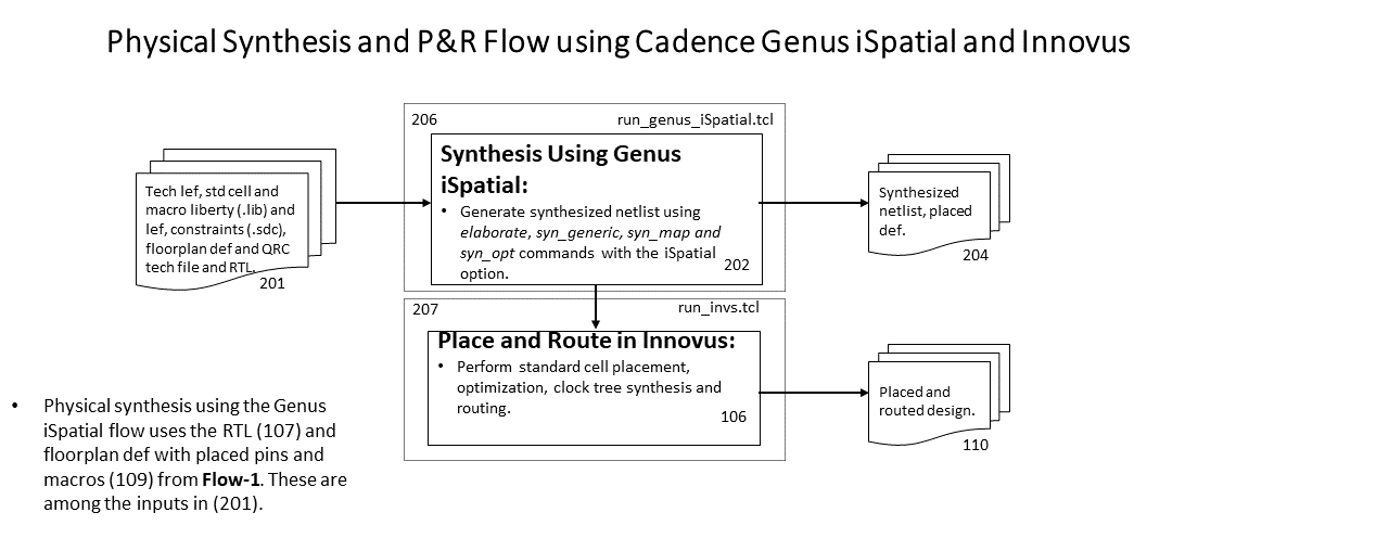
Question 12. How well does Simulated Annealing (SA) optimize the proxy cost?
Details of our SA implementation, which we denote as SA-UCSD, are here. We have used SA-UCSD to generate macro placements for Ariane and BlackParrot (Quad-Core). We find that SA-UCSD produces better proxy costs than CT.
- Ariane133-NG45-68%-1.3ns: The configuration that results best proxy cost (wirelength cost: 0.0881, congestion cost: 0.8257, density cost: 0.5084, proxy cost: 0.75515): action_probs: [0.2, 0.2, 0.2, 0.2, 0.2], num_actions: 3, max_temperature: 7e-5, num_iters: 50000, seed: 1, spiral_flag: True
- The following table and screenshots provide details of Ariane133-NG45-68%-1.3ns SA-UCSD macro placement.
| Ariane133-NG45-68%-1.3ns SA-UCSD result (Link to CT result) (Link to CMP result) | |||||||||
|---|---|---|---|---|---|---|---|---|---|
| Physical Design Stage | Core Area (um^2) | Standard Cell Area (um^2) | Macro Area (um^2) | Total Power (mW) | Wirelength (um) | WS (ns) | TNS (ns) | Congestion (H) | Congestion (V) |
| preCTS | 1814274 | 243604 | 1018356 | 786.182 | 3825529 | -0.130 | -187.073 | 0.01% | 0.03% |
| postCTS | 1814274 | 245443 | 1018356 | 827.698 | 3868208 | -0.099 | -52.565 | 0.02% | 0.06% |
| postRoute | 1814274 | 245443 | 1018356 | 827.546 | 3982401 | -0.125 | -114.924 | ||
| postRouteOpt | 1814274 | 245804 | 1018356 | 828.053 | 3986262 | -0.112 | -75.338 | ||


- BlackParrot (Quad-Core)-NG45-68%-1.3ns: The configuration that results best proxy cost (wirelength cost: 0.0604, congestion cost: 0.9581, density cost: 0.7383, proxy cost: 0.90860): action_probs: [0.2, 0.2, 0.2, 0.2, 0.2], num_actions: 1, max_temperature: 10e-5, num_iters: 20000, seed: 1, spiral_flag: False
- The following table and screenshots provide details of BlackParrot (Quad-Core)-NG45-68%-1.3ns SA-UCSD macro placement.
| BlackParrot Quad-Core-NG45-68%-(bp clock)1.3ns SA-UCSD (Link to CT result) (Link to CMP result) | |||||||||
|---|---|---|---|---|---|---|---|---|---|
| Physical Design Stage | Core Area (um^2) | Standard Cell Area (um^2) | Macro Area (um^2) | Total Power (mW) | Wirelength (um) | WS (ns) | TNS (ns) | Congestion (H) | Congestion (V) |
| preCTS | 8449457 | 1921810 | 3917822 | 4185.031 | 30470310 | -0.209 | -863.535 | 0.08% | 0.32% |
| postCTS | 8449457 | 1934844 | 3917822 | 4560.519 | 30568687 | -0.107 | -267.191 | 0.09% | 0.36% |
| postRoute | 8449457 | 1934844 | 3917822 | 4539.416 | 31510301 | -0.239 | -6022.700 | ||
| postRouteOpt | 8449457 | 1943841 | 3917822 | 4547.886 | 31550599 | -0.222 | -3263.800 | ||


Question 13. How good are human macro placements relative to Circuit Training?
We observe that human macro placements can achieve smaller wirelength than CT, with similar timing and power numbers. Details of human macro placements for BlackParrot (Quad-Core) and MemPool Group on NG45 enablement are as follows:
- BalckParrot-NG45-68%-1.3ns: We thank Dr. Jinwook Jung of IBM Research for providing his human macro placement of BlackParrot Quad-Core design as an alternative baseline. The following table and screenshots provide details of BlackParrot (Quad-Core)-NG45-68%-1.3ns human macro placement. Link to the script.
- Dr. Jung informed us that he spent about 0.5 hours learning about the design, 2.5 hours coming up with initial floorplan scripts, and an additional 2.5 hours refining the initial version, for a total of 5.5 hours of effort. Dr. Jung also informed us that his floorplan design includes 4 identical tiles, and that these are arranged so as to create more free space.
| BlackParrot Quad-Core-NG45-68%-1.3ns Human macro placement (not a gridded placement) (Link to CT result) (Link to CMP result) | |||||||||
|---|---|---|---|---|---|---|---|---|---|
| Physical Design Stage | Core Area (um^2) | Standard Cell Area (um^2) | Macro Area (um^2) | Total Power (mW) | Wirelength (um) | WS (ns) | TNS (ns) | Congestion (H) | Congestion (V) |
| preCTS | 8449457 | 1907164 | 3917822 | 4107.931 | 24814112 | -0.195 | -530.552 | 0.08% | 0.12% |
| postCTS | 8449457 | 1918983 | 3917822 | 4475.523 | 24944903 | -0.097 | -209.587 | 0.09% | 0.13% |
| postRoute | 8449457 | 1918983 | 3917822 | 4468.904 | 25888999 | -0.120 | -454.561 | ||
| postRouteOpt | 8449457 | 1919928 | 3917822 | 4469.552 | 25915520 | -0.097 | -321.918 | ||


- MemPool Group-NG45-68%-4ns: The following macro placement is generated by Sayak Kundu based on the tile configuration received from Matheus Cavalcante, ETH Zürich and Jiantao Liu. Link to the MemPool Group macro placement script. The following table and screenshots provide details of MemPool Group-NG45-68%-4ns human macro placement.
| MemPool Group-NG45-68%-4ns human macro placement (not a gridded placement) (Link to CT result) (Link to CMP result) | |||||||||
|---|---|---|---|---|---|---|---|---|---|
| Physical Design Stage | Core Area (um^2) | Standard Cell Area (um^2) | Macro Area (um^2) | Total Power (mW) | Wirelength (um) | WS (ns) | TNS (ns) | Congestion (H) | Congestion (V) |
| preCTS | 11371934 | 4930345 | 3078071 | 2459.392 | 101645170 | -0.021 | -141.801 | 0.39% | 0.86% |
| postCTS | 11371934 | 4883741 | 3078071 | 2640.242 | 102110339 | -0.003 | -0.055 | 0.58% | 0.96% |
| postRoute | 11371934 | 4883741 | 3078071 | 2642.017 | 107463344 | -0.246 | -2941.400 | ||
| postRouteOpt | 11371934 | 4873872 | 3078071 | 2639.916 | 107597894 | -0.049 | -11.897 | ||


We have also added
- Ariane133-NG45-68%-1.3ns: Link to the human macro placement details of Ariane on NG45 enablement.
- MemPool Group-GF12-68%: Link to the human macro placement details of MemPool Group on GF12 enablement.
March 5:
Question 14. What is the impact on CT results when DREAMPlace is used instead of force-directed placement?
We have integrated DREAMPlace in Circuit Training (commit hash: 91e14fd1caa5b15d9bb1b58b6d5e47042ab244f3) and trained CT to generate macro placement solutions for Ariane, BlackParrot and MemPool Group designs. We referer to CT with DREAMPlace as CT+DREAMPlace and CT with FD as CT+FD. The training results are as follows:
- Ariane133-NG45-68%-1.3ns: Following table and screenshots presents the macro placement solution generated by CT+DREAMPlace for Ariane133 design with 68% floorplan utilization, 1.3ns target clock period on NG45 enablement. (Wirelength Cost:0.0678, Congestion cost: 0.8320, Density cost: 0.5239)
Ariane133-NG45-68%-1.3ns CT+DREAMPlace result (Link to tensorboard) (Link to CT+FD result) |
|||||||||
|---|---|---|---|---|---|---|---|---|---|
| Physical Design Stage | Core Area (um^2) | Standard Cell Area (um^2) | Macro Area (um^2) | Total Power (mW) | Wirelength (um) | WS (ns) | TNS (ns) | Congestion (H) | Congestion (V) |
| preCTS | 1814274 | 244313 | 1018356 | 791.482 | 4669338 | -0.135 | -176.306 | 0.05% | 0.12% |
| postCTS | 1814274 | 244976 | 1018356 | 830.645 | 4693972 | -0.106 | -75.708 | 0.05% | 0.15% |
| postRoute | 1814274 | 244976 | 1018356 | 828.923 | 4822561 | -0.124 | -109.91 | ||
| postRouteOpt | 1814274 | 245438 | 1018356 | 829.353 | 4827641 | -0.126 | -93.752 | ||


- BlackParrot(Quad-Core)-NG45-68%-1.3ns: Following table and screenshots presents the macro placement solution generated by CT+DREAMPlace for BlackParrot design with 68% floorplan utilization, 1.3ns target clock period on NG45 enablement. (Wirelength cost: 0.0878, Density cost: 0.5687, Congestion cost: 1.1420)
BP(Quad-Core)-NG45-68%-1.3ns CT+DREAMPlace (Link to tensor board) (Link to CT+FD result) |
|||||||||
|---|---|---|---|---|---|---|---|---|---|
| Physical Design Stage | Core Area (um^2) | Standard Cell Area (um^2) | Macro Area (um^2) | Total Power (mW) | Wirelength (um) | WS (ns) | TNS (ns) | Congestion (H) | Congestion (V) |
| preCTS | 8449457 | 1959789 | 3917822 | 4396.086 | 42267061 | -0.209 | -1132.2 | 0.28% | 0.57% |
| postCTS | 8449457 | 1978100 | 3917822 | 4783.785 | 42346079 | -0.163 | -680.8 | 0.29% | 0.63% |
| postRoute | 8449457 | 1978100 | 3917822 | 4751.075 | 43883402 | -0.201 | -1406.3 | ||
| postRouteOpt | 8449457 | 1979794 | 3917822 | 4753.696 | 43931174 | -0.178 | -850.8 | ||


- MemPool Group-NG45-68%-1.3ns: Following table and screenshots presents the macro placement solution generated by CT+DREAMPlace for MemPool Group design with 68% floorplan utilization, 4ns target clock period on NG45 enablement. (Wirelength cost: 0.0728, Density cost: 0.6617, Congestion cost: 1.2714) DRC Count: 14779.
MemPool Group-NG45-68%-4ns CT+DREAMPlace (Link to tensorboard) (Link to CT+FD Result) |
|||||||||
|---|---|---|---|---|---|---|---|---|---|
| Physical Design Stage | Core Area (um^2) | Standard Cell Area (um^2) | Macro Area (um^2) | Total Power (mW) | Wirelength (um) | WS (ns) | TNS (ns) | Congestion (H) | Congestion (V) |
| preCTS | 11371934 | 4990302 | 3078071 | 2659.403 | 121635791 | -0.015 | -71.824 | 3.33% | 3.26% |
| postCTS | 11371934 | 4969651 | 3078071 | 2839.139 | 122062712 | -0.004 | -0.104 | 3.49% | 3.19% |
| postRoute | 11371934 | 4969651 | 3078071 | 2893.588 | 132078512 | -1.137 | -29243.4 | ||
| postRouteOpt | 11371934 | 4995348 | 3078071 | 2908.959 | 132299696 | -0.072 | -97.892 | ||


Question 15. Should we factor in density cost while using DREAMPlace for CT?
We update the density weight from 0.5 to 0.0, then rerun CT-DREAMPlace for Ariane, BlackParrot and MemPool Group designs. The training results are as follows:
- Ariane133-NG45-68%-1.3ns: Following table and screenshots presents the macro placement solution generated by CT+DREAMPlace for Ariane133 design with 68% floorplan utilization, 1.3ns target clock period on NG45 enablement when density weight is 0. (Wirelength Cost: 0.0715, Congestion cost: 0.8111, Density cost: 0.5251)
Ariane133-NG45-68%-1.3ns CT+DREAMPlace result (Density Weight = 0.0) (Link to tensorboard) (Link to CT+FD result) |
|||||||||
|---|---|---|---|---|---|---|---|---|---|
| Physical Design Stage | Core Area (um^2) | Standard Cell Area (um^2) | Macro Area (um^2) | Total Power (mW) | Wirelength (um) | WS (ns) | TNS (ns) | Congestion (H) | Congestion (V) |
| preCTS | 1814274 | 245097 | 1018356 | 793.171 | 4959656 | -0.137 | -202.147 | 0.04% | 0.17% |
| postCTS | 1814274 | 248172 | 1018356 | 839.062 | 4993255 | -0.117 | -108.074 | 0.04% | 0.15% |
| postRoute | 1814274 | 248172 | 1018356 | 836.985 | 5114089 | -0.164 | -243.834 | ||
| postRouteOpt | 1814274 | 248775 | 1018356 | 837.655 | 5119513 | -0.16 | -152.043 | ||


- BlackParrot(Quad-Core)-NG45-68%-1.3ns: Following table and screenshots presents the macro placement solution generated by CT+DREAMPlace for BlackParrot design with 68% floorplan utilization, 1.3ns target clock period on NG45 enablement when density weight is 0. (Wirelength cost: 0.0791, Density cost: 0.5770, Congestion cost: 1.0964)
BP(Quad-Core)-NG45-68%-1.3ns CT+DREAMPlace (Density weight = 0.0) (Link to tensorboard) (Link to CT+FD result) |
|||||||||
|---|---|---|---|---|---|---|---|---|---|
| Physical Design Stage | Core Area (um^2) | Standard Cell Area (um^2) | Macro Area (um^2) | Total Power (mW) | Wirelength (um) | WS (ns) | TNS (ns) | Congestion (H) | Congestion (V) |
| preCTS | 8449457 | 1947589 | 3917822 | 4323.518 | 38208933 | -0.233 | -1177.6 | 0.33% | 0.46% |
| postCTS | 8449457 | 1961564 | 3917822 | 4703.800 | 38314312 | -0.153 | -468.3 | 0.37% | 0.49% |
| postRoute | 8449457 | 1961564 | 3917822 | 4674.250 | 39753854 | -0.200 | -1995.5 | ||
| postRouteOpt | 8449457 | 1964239 | 3917822 | 4677.048 | 39800843 | -0.180 | -809.0 | ||


- MemPool Group-NG45-68%-1.3ns: Following table and screenshots presents the macro placement solution generated by CT+DREAMPlace for MemPool Group design with 68% floorplan utilization, 4ns target clock period on NG45 enablement when density weight is 0. (Wirelength cost: 0.0711, Density cost: 0.6666, Congestion cost: 1.2605 ) DRC Count: 3260
MemPool Group-NG45-68%-4ns CT+DREAMPlace (Density weight = 0.0) (Link to tensorboard) (Link to CT+FD Result) |
|||||||||
|---|---|---|---|---|---|---|---|---|---|
| Physical Design Stage | Core Area (um^2) | Standard Cell Area (um^2) | Macro Area (um^2) | Total Power (mW) | Wirelength (um) | WS (ns) | TNS (ns) | Congestion (H) | Congestion (V) |
| preCTS | 11371934 | 4934839 | 3078071 | 2613.613 | 119923841 | -0.027 | -146.5 | 2.56% | 2.51% |
| postCTS | 11371934 | 4928559 | 3078071 | 2802.851 | 120508367 | -0.003 | -0.1 | 2.87% | 2.66% |
| postRoute | 11371934 | 4928559 | 3078071 | 2848.873 | 130024068 | -0.803 | -19920.7 | ||
| postRouteOpt | 11371934 | 4953483 | 3078071 | 2858.071 | 130243153 | -0.050 | -33.5 | ||


We observe from the above results that CT+DREAMPlace achieves similar result for density weight 0 and 0.5.
Question 16. Why does your study (and, ISPD-2023 paper) use Cadence CMP 21.1, which was not available to Google engineers when they wrote the Nature paper?
We used Innovus version 21.1 since it was the latest version of our place-and-route evaluator of macro placement solutions. CMP 21.1 is part of Innovus 21.1. Using the latest version of CMP was also natural, given our starting assumption that RL from Nature would outperform the commercial state-of-the-art.
We have now run further experiments using older versions of CMP and Innovus. We find that the macro placements produced by CMP across versions 19.1, 20.1 and 21.1 lead to the same qualitative conclusions. Additional details:
- The Concurrent Macro Placer (CMP) was available in both the 19.1 and 20.1 versions of Cadence Innovus. Our published flow scripts can also be used to run Innovus 19.1 and 20.1 with a few lines commented out: lines1 and lines2.
- For the Ariane133-NG45-68%-1.3ns testcase, we have run CMP + Innovus in two additional Cadence releases (19.1, 20.1). This corresponds to Steps “4” and “5” of the industrial evaluation flow in Figure 2 of our paper, and a “pure commercial tool flow”.
- We assess the CT macro placement that is reported in Table 1 of our ISPD-2023 paper, using all three Innovus P&R versions. The CT post-P&R results are inferior to those obtained with corresponding CMP versions.
- This new study reinforces the conclusion obtained using CMP + Innovus (21.1) in our paper. This can be independently verified using provided scripts. We do not provide additional numbers, in order to avoid benchmarking of the Cadence tool versions.
Below are screenshots of Ariane-NG45-68%-1.3ns for (in order, top-down) CMP + P&R outcomes in Innovus 19.1, 20.1 and 21.1 versions.
- Ariane133-NG45-68%-1.3ns (CMP + Innovus 19.1)


- Ariane133-NG45-68%-1.3ns (CMP + Innovus 20.1)


- Ariane133-NG45-68%-1.3ns (CMP + Innovus 21.1 is the same as in Figure 3 of our paper)

- Left to right: CT macro placement from the ISPD-2023 paper, with P&R using Innovus 19.1, 20.1 and 21.1. (21.1 is the same as in Figure 3 of our paper.)


Question 17. What are the outcomes of CT when the training is continued until convergence?
To put this question in perspective, training “until convergence” is not described in any of the guidelines provided by the CT GitHub repo for reproducing the results in the Nature paper. For the ISPD 2023 paper, we adhere to the guidelines given in the CT GitHub repo, use the same number of iterations for Ariane as Google engineers demonstrate in the CT GitHub repo, and obtain results that closely align with Google’s outcomes for Ariane. (See FAQs #4 and #13.)
We run CT training for an extended number (=600) of iterations, for each of Ariane, BlackParrot and MemPool Group on NG45, and make the following observations.
- For Ariane the proxy cost improves from 0.857 to 0.809 (link to the new tensorboard). However, the Nature Table 1 metrics are very similar: routed wirelength improves from 4,894mm to 4,739mm; Total power degrades from 828.7 mW to 829.4 mW; worst negative slack and total negative slack respectively degrade from -79ps to -85ps, and from -25.8ns to -62.7ns. The final proxy cost and the Nature Table 1 metrics achieved through training until convergence are still not better than those achieved by SA.
- For BlackParrot, the proxy cost improves significantly from 1.021 to 0.889 (link to new tensorboard). Routed wirelength improves significantly from 36,845mm to 30,929mm. Also total power improves from 4627.4mW to 4547.8mW. However, the worst negative slack and total negative slack respectively degrade from -185ps to -199ps, and from -1040.8ns to -1263.4ns. The final proxy cost achieved by CT is better than that achieved by SA. The Nature Table 1 metrics are still similar to those achieved by SA.
- For MemPool Group, CT diverges, and it never converges. Thus, the final proxy cost is unchanged. Here is the link to tensorboard. So, the CT code does not guarantee full convergence.
- Note 1: We have not studied what happens if SA is given triple the runtime used in our previously-reported experiments.
- Note 2: Our new data underscore the poor correlation between proxy cost and ground-truth metrics noted in Section 5.2.3 of the ISPD-2023 paper.
Our new data from using triple the CT training budget indicate that training until convergence, compared to the configurations explored in the ISPD-2023 paper, improves proxy cost but does not significantly improve chip metrics on Ariane and MemPool Group. Among chip metrics for BlackParrot, routed wirelength improves significantly while other metrics are similar to what we previously reported. Overall, training until convergence does not qualitatively change comparisons to results of Simulated Annealing and human macro placements reported in the ISPD 2023 paper.
The subsequent tables and figures present the Nature Table 1 metrics of Ariane and BlackParrot on NG45, for macro placement solutions generated by CT training until convergence. (For MemPool Group, using triple the default number of CT iterations did not change the final proxy cost.)
Ariane133-NG45-68%-1.3ns CT result (Link to tensorboard) |
|||||||||
|---|---|---|---|---|---|---|---|---|---|
| Physical Design Stage | Core Area (um^2) | Standard Cell Area (um^2) | Macro Area (um^2) | Total Power (mW) | Wirelength (um) | WS (ns) | TNS (ns) | Congestion(H) | Congestion (V) |
| preCTS | 1814274 | 242539 | 1018356 | 787.798 | 4577259 | -0.095 | -121.911 | 0.04% | 0.11% |
| postCTS | 1814274 | 244220 | 1018356 | 830.273 | 4610696 | -0.07 | -41.635 | 0.05% | 0.13% |
| postRoute | 1814274 | 244220 | 1018356 | 828.935 | 4734768 | -0.095 | -90.160 | ||
| postRouteOpt | 1814274 | 244666 | 1018356 | 829.419 | 4739136 | -0.085 | -62.685 | ||


BlackParrot (Quad-Core)-NG45-68%-1.3ns CT result (Link to tensorboard) |
|||||||||
|---|---|---|---|---|---|---|---|---|---|
| Physical Design Stage | Core Area (um^2) | Standard Cell Area (um^2) | Macro Area (um^2) | Total Power (mW) | Wirelength (um) | WS (ns) | TNS (ns) | Congestion (H) | Congestion (V) |
| preCTS | 8449457 | 1922798 | 3917822 | 4185.939 | 29820259 | -0.179 | -648.911 | 0.10% | 0.26% |
| postCTS | 8449457 | 1935706 | 3917822 | 4563.875 | 29956480 | -0.138 | -355.347 | 0.12% | 0.28% |
| postRoute | 8449457 | 1935706 | 3917822 | 4542.299 | 30893195 | -0.188 | -2280.100 | ||
| postRouteOpt | 8449457 | 1940957 | 3917822 | 4547.832 | 30928844 | -0.199 | -1263.400 | ||


Question 18. To study the benefit that CT derives from use of a commercial placement solution, why do you compare with giving CT “impossible” initial placements, where all instances are placed at the same location?
- Section 5.2.1 of our ISPD-2023 paper discusses the advantage that CT derives from its use of initial placement information from a commercial EDA tool. To measure this advantage, we study what happens when CT is deprived of this placement information.
- In Question 1, August 2022 we used “vacuous” placements where the same (x,y) location is given for all instances. This corresponds to the use of placements that have as little information content as possible. However, after publication of our ISPD-2023 paper, comments were made that such placements are “impossible”.
- We have now performed a second study that gradually perturbs the EDA tool’s placement and measures the effect on CT outcomes. In this second study, we always maintain legal placements: every placement that is fed to CT is “possible”. Our new study directly assesses how CT’s performance changes as the commercial EDA tool’s placement is degraded.
- Note 1: CT’s grouping flow requires (x,y) coordinates in the input.
- Note 2: We cannot use a “random, but possible” placement as input to CT. This leads to a blowup of the numbers of clusters and edges in the adjacency matrix. [E.g.: “IndexError: index 3500 is out of bounds for axis 0 with size 3500” from CT. There is also a default limit of 42000 edges in CT.]
- The gen_perturbed_placement procedure below randomly perturbs the original placement solution from commercial physical synthesis, by shuffling the placed locations of a prescribed fraction of instances in the design. (E.g., when the parameter x = 0.05, the locations of 5% of the netlist will be shuffled.)
Procedure gen_perturbed_placement
Input: seed, x
# x indicates the fraction of instances to be moved 0 < x < 1.0
1. For w, h in {unique list of instance (width, height)}
  a. instance_list = {list of instances with width = w and height = h}
  b. instance_list = shuffle(instance_list, seed)
  c. instance_count = length(shuffled_instance_list)
  d. shuffled_instance_list = instance_list[:instance_count*x]
  e. shuffle_placement(shuffled_instance_list, seed)
Procedure shuffle_placement
Input: instance_list, seed
1. X, Y, Orient = {list of lower left coordinate and orientation of instances in the instance_list}
2. shuffled_instance_list = shuffle(instance_list, seed)
3. For i in range(length(instance_list)):
  a. Update location and orientation of shuffled_instance_list[i] with (X[i], Y[i]) and Orient[i]
- The table below shows what happens as the commercial EDA tool’s “possible” initial placement is degraded into other “possible” initial placements, for all combinations of x = {0.01, 0.05, 0.15} and seed = {21, 42, 63}. The value x = 0.0 corresponds to the CT outcome that we report in Table 1 of our ISPD-2023 paper. We include the “Human” and “SA” rows from our Table 1 for ease of reference.
- From the data, we observe that degrading the commercial placement information worsens all CT outcomes except for routed wirelength across all seed values. Runtime is also worsened, e.g., with x = 0.15 the CT runtime in our environment was 52.0 hours which is 1.6 times longer than when x = 0.0 (See #13 of our FAQs.). This is at least in part because having more moving elements (soft macros) increases CT’s runtime in force-directed placement and proxy cost evaluation.
- For the nine perturbed placements, SA yields better proxy cost and chip metrics compared to CT in most cases.
- Note 3: We have not studied what happens if SA is given 1.6 times the runtime used in our previously-reported experiments.

April 27, 2023:
We have run Hier-RTLMP macro placer, as described in the arXiv paper, on our modern benchmarks. The code for Hier-RTLMP is open-sourced here. We use the default settings to generate the macro placement solutions. The results are as follows:
- Ariane133-NG45-68%-1.3ns: Following table and screenshots show the macro placement result of Ariane133 on NG45, generated using Hier-RTLMP.
Ariane133-NG45-68%-1.3ns Hier-RTLMP (Link to CT result) (Link to CMP result) |
|||||||||
|---|---|---|---|---|---|---|---|---|---|
| Physical Design Stage | Core Area (um^2) | Standard Cell Area (um^2) | Macro Area (um^2) | Total Power (mW) | Wirelength (um) | WS (ns) | TNS (ns) | Congestion (H) | Congestion (V) |
| preCTS | 1814274 | 246916 | 1018356 | 796.781 | 5087055 | -0.149 | -192.7 | 0.11% | 0.08% |
| postCTS | 1814274 | 247403 | 1018356 | 836.595 | 5136058 | -0.110 | -104.2 | 0.15% | 0.10% |
| postRoute | 1814274 | 247403 | 1018356 | 835.096 | 5291106 | -0.178 | -356.0 | ||
| postRouteOpt | 1814274 | 248296 | 1018356 | 836.002 | 5296879 | -0.165 | -223.4 | ||


-
Ariane133-GF12-68%: Link to the HierRTLMP macro placement details of Ariane on GF12 enablement.
-
BlackParrot (Quad-Core)-NG45-68%-1.3ns: Following table and screenshots show the macro placement result of BlackParrot (Quad-Core) on NG45, generated using Hier-RTLMP.
BlackParrot-NG45-68%-1.3ns Hier-RTLMP (Link to CT result) (Link to CMP result) |
|||||||||
|---|---|---|---|---|---|---|---|---|---|
| Physical Design Stage | Core Area (um^2) | Standard Cell Area (um^2) | Macro Area (um^2) | Total Power (mW) | Wirelength (um) | WS (ns) | TNS (ns) | Congestion (H) | Congestion (V) |
| preCTS | 8449457 | 1908372 | 3917822 | 4148.534 | 27687847 | -0.169 | -455.5 | 0.13% | 0.17% |
| postCTS | 8449457 | 1923367 | 3917822 | 4522.966 | 27810361 | -0.123 | -181.5 | 0.15% | 0.20% |
| postRoute | 8449457 | 1923367 | 3917822 | 4509.596 | 28835670 | -0.166 | -906.8 | ||
| postRouteOpt | 8449457 | 1925012 | 3917822 | 4511.780 | 28865504 | -0.150 | -456.6 | ||


-
BlackParrot (Quad-Core)-GF12-68%: Link to the HierRTLMP macro placement details of BlackParrot (Quad-Core) on GF12 enablement.
-
MemPool Group-NG45-68%-4ns: Following table and screenshots show the macro placement result of MemPool Group on NG45, generated using Hier-RTLMP.
MemPool Group-NG45-68%-4ns Hier-RTLMP (62 DRCs) (Link to CT result) (Link to CMP result) |
|||||||||
|---|---|---|---|---|---|---|---|---|---|
| Physical Design Stage | Core Area (um^2) | Standard Cell Area (um^2) | Macro Area (um^2) | Total Power (mW) | Wirelength (um) | WS (ns) | TNS (ns) | Congestion (H) | Congestion (V) |
| preCTS | 11371934 | 4939447 | 3078071 | 2489.1 | 105739299 | -0.016 | -50.5 | 2.05% | 1.03% |
| postCTS | 11371934 | 4895581 | 3078071 | 2671.4 | 106267958 | -0.002 | -0.1 | 2.31% | 1.18% |
| postRoute | 11371934 | 4895581 | 3078071 | 2696.2 | 113924593 | -0.503 | -4743.7 | ||
| postRouteOpt | 11371934 | 4889459 | 3078071 | 2695.3 | 114073113 | -0.062 | -4.9 | ||


- MemPool Group-GF12-68%: Link to the HierRTLMP macro placement details of MemPool Group on GF12 enablement.
Protobuf to LEF/DEF and macro placement of CT-Ariane
We have released a new Protobuf-to-LEF/DEF translator in our repository;
detailed information is available in
CodeElements/FormatTranslators.
Using this translator, we have generated LEF/DEF files from the
Protobuf netlist
of the Ariane design (the only publicly available design disclosed by the
authors of the Nature paper) available in the Circuit Training repository.
We believe that, consistent with the sub-10nm characterization of testcases
mentioned in the Nature paper, CT-Ariane corresponds to an implementation in
TSMC 7nm technology. This belief is based on two aspects of the Protobuf netlist
posted by Google Brain. (1) First, in the Protobuf header, we see
“ariane_tsmc7_dc_09162019”, which suggests that the design is in the TSMC 7nm
node. (2) Second, we find here that in TSMC 7nm technology, the standard-cell
height is either 240nm or 300nm. All single-height standard cells in the
CT-Ariane Protobuf posted by Google Brain have a height of 240nm (i.e., “HD”).
The cell naming seen in Google’s posted Ariane testcase (e.g.,
“NR2D1BWP240H8P57PDSVT”) matches conventions commonly seen with TSMC-based
design enablement.
With these generated LEF/DEF files, we have created macro placement solutions using Circuit Training (CT), RePlAce, and Innovus Concurrent Macro Placer (CMP). To evaluate these macro placement solutions, we use Innovus21.1. The evaluation flow is as follows: (1) we first legalize macro placement solutions using the refine_macro_place command; (2) we then place standard cells using the place_design command; and (3) finally, we report post-placement HPWL.
The figure below shows visualizations of the macro placement solutions generated by Circuit Training (commit hash: 1e14fd1ca), RePlAce (OpenROAD, commit hash: ad808fd, command: global_placement -density 0.8) and Innovus CMP (version: 21.1, command: place_design -concurrent_macros) for the CT-Ariane (original, “X1”) Protobuf. The corresponding LEF/DEF files are here. Please note that we report this data as part of our study of Circuit Training. It is not intended to “benchmark” any commercial EDA tool in any sense, and the data should not be interpreted as providing any sort of “benchmarking” comparison or value judgment regarding the commercial tool.
 |
|  |
|  |
| **HPWL:** 1,117,300µm
|
| **HPWL:** 1,117,300µm**Runtime:** ~112,824s
(using 8 NVIDIA-V100 GPUs,
96 CPU threads, 354 GB RAM) | **HPWL:** 922,344µm
**Runtime:** 81s
(using 1 thread) | **HPWL:** 746,816µm
**Runtime:** 294s
(Innovus launched with 8 threads) |
We have scaled the Protobuf netlist of the Ariane design in the Circuit Training repository into CT-Ariane-X2 and CT-Ariane-X4, following the “quantified suboptimality” studies in the DAC-1995 paper, “Quantified suboptimality of VLSI layout heuristics”. For a given testcase, self-scaling of additional copies can be performed in two basic ways: shift and flip.
- The shift operation translates a given copy along the X and/or Y axis, relative to the original testcase.
- The flip operation mirrors the given copy about the X or Y axis.
By combining these actions, it is possible to obtain variants of the X2 design using X-Shift (the second copy is placed to the right of the original copy), Y-Shift (the second copy is placed above the original copy), X-Flip (the second copy mirrors the original copy about the X axis), and Y-Flip (the second copy mirrors the original copy about the Y axis). Variants for the X4 design can be obtained by serial application of these actions, e.g., X-Shift-Y-Shift, X-Flip-Y-Flip, X-Shift-Y-Flip, X-Flip-Y-Shift, etc. However, considering that all I/O pins must be placed at the boundaries, two variants are of more interest for CT-Ariane-X4: X-Shift-Y-Flip and X-Flip-Y-Flip.
Our naming convention is as follows: CT-Ariane-X4-X-Shift-Y-Flip indicates a design that is an X4 version of the original CT-Ariane design. It is generated by first shifting the X1 copy along the X-axis to obtain an X2 copy, then flipping the X2 copy along the Y-axis to create the X4 copy. For the CT-Ariane-X2, we generate two versions: CT-Ariane-X2-Y-Flip and CT-Ariane-X2-X-Shift. For the CT-Ariane-X4, we generate two versions: CT-Ariane–X4-X-Shift-Y-Flip and CT-Ariane-X4-X-Flip-Y-Flip.
The following figures show visualizations of the macro placement solutions for each version, generated using RePlAce (OpenROAD, commit hash: ad808fd) and Innovus CMP (version 21.1). HPWL and runtime values are also shown. The detailed command and evaluation flow are the same as those used for the original CT-Ariane (X1) study.
X2 Versions: (CT-Ariane-X2-Y-Flip)
 |
|  |
| **HPWL:** 1,851,241µm
|
| **HPWL:** 1,851,241µm**Runtime:** 170s | **HPWL:** 1,510,131µm
**Runtime:** 534s |
X2 Versions: (CT-Ariane-X2-X-Shift)
 |
|  |
| **HPWL:** 1,901,242µm
|
| **HPWL:** 1,901,242µm**Runtime:** 193s | **HPWL:** 1,513,938µm
**Runtime:** 597s |
X4 Versions: (CT-Ariane-X4-X-Shift-Y-Flip)
 |
|  |
| **HPWL:** 3,700,397µm
|
| **HPWL:** 3,700,397µm**Runtime:** 361s | **HPWL:** 3,051,941µm
**Runtime:** 1,357s |
X4 Versions: (CT-Ariane-X4-X-Flip-Y-Flip)
 |
|  |
| **HPWL:** 3,742,491µm
|
| **HPWL:** 3,742,491µm**Runtime:** 372s | **HPWL:** 3,046,270µm
**Runtime:** 1,262s |
| Design (Iterations) |
CT-Scratch | CT-AC | CT-Ours | |||
|---|---|---|---|---|---|---|
| 200 | 400 | 200 | 400 | 200 | 400 | |
| Ariane-NG45 | Link | Link | Link+ | Link | Link+ | |
| BlackParrot-NG45 | Link+ | Link | Link+ | |||
| MemPoolGroup-NG45 | Link | Link+ | Link | Link+ | ||
| Ariane-ASAP7 | Link | Link+ | Link | Link | Link+ | |
| BlackParrot-ASAP7 | Link+ | Link | Link+ | |||
| MemPoolGroup-ASAP7 | Link+ | Link | Link+ | |||
| Ariane-GF12 | Link | Link | Link | Link+ | ||
| BlackParrot-GF12 | Link+ | Link+ | ||||
| MemPoolGroup-GF12 | Link | Link+ | Link | Link+ | ||
| CT-Ariane | Link | Link+ | Link | Link+ | ||
| CT-Ariane-X2 | Link | Link+ | ||||
| CT-Ariane-X4 | Link | Link+ | ||||
| Technology | Ariane | MemPoolGroup | |
|---|---|---|---|
| NG45 | Link | (Shift, X/Y/XY-flip, Shift-X/Y/XY-flip) Link (Shift, XY-flip, Shift-X/Y/XY-flip) Link (Shift, X/Y-flip, Shift-X/Y-flip) Link (Shift, X/Y-flip, Shift-XY-flip) Link (Shift, X/Y-flip) Link |
|
| ASAP7 | Link | ||
| GF12 | Link | (Shift, X/Y/XY-flip, Shift-X/Y/XY-flip) Link (Shift, XY-flip, Shift-X/Y/XY-flip) Link (Shift, X/Y-flip, Shift-X/Y-flip) Link (Shift, X/Y-flip, Shift-XY-flip) Link (Shift, X/Y-flip) Link |
|
| CT-Ariane | CT-Ariane-X2 | CT-Ariane-X4 | |
| TSMC N7 | Link | Link | (CT-Ariane-X1-{Shift, X/Y-flip}, CT-Ariane-X2-{Shift, X/Y-flip}) Link (CT-Ariane-X4) Link |
| Seed | RUN 1 | RUN 2 | RUN 3 | |||
|---|---|---|---|---|---|---|
| 111 | Link | Link+ | Link | Link+ | Link | Link+ |
| 222 | Link | Link+ | Link | Link+ | Link | Link+ |
| 333 | Link | Link+ | Link | Link+ | Link | Link+ |
| Lower Left | Center | Upper Right | No Placement |
|---|---|---|---|
| Link | Link | Link | Link |
| Link+ | Link+ | Link+ | Link+ |